What Is Macroeconomics

Macroeconomics is the study of the economy as a whole. Rather than focusing on the behaviour of individual households, individual firms, or individual markets, macroeconomics examines how the entire economic system operates and how its main variables are related to one another. These variables include total output, total income, total expenditure, employment, unemployment, inflation, and economic growth.

The defining feature of macroeconomics is its use of aggregate variables. An aggregate variable is a total measure that combines the behaviour of many individual economic units into a single economy-wide value. For example, instead of analysing the wage earned by one worker, macroeconomics considers the total wages paid to all workers in the economy. Instead of examining the output of one firm, it considers the total value of all goods and services produced across the entire economy over a given period of time.

This focus on aggregates allows macroeconomics to address questions that cannot be answered through microeconomic analysis alone. Questions such as why unemployment rises during recessions, why inflation accelerates in some periods but not others, or why economic growth differs across time all require an economy-wide perspective. Macroeconomics therefore complements microeconomics rather than replacing it. Microeconomics explains how individual markets work, while macroeconomics explains how those markets fit together to determine overall economic outcomes.

In macroeconomic analysis, it is important to distinguish between individual outcomes and economy-wide outcomes. For example, one person losing a job is a microeconomic issue, whereas a sustained increase in the national unemployment rate is a macroeconomic issue. Similarly, a rise in the price of one product is a microeconomic concern, while a general rise in the overall price level across the economy is a macroeconomic phenomenon known as inflation.

Another defining feature of macroeconomics is its emphasis on relationships between variables. Macroeconomists are less concerned with isolated outcomes and more concerned with how changes in one variable affect others. For example, macroeconomics examines the relationship between income and consumption, between investment and interest rates, and between aggregate demand and the overall price level. Understanding these relationships is essential for explaining how economies respond to shocks and how policy interventions may alter economic performance.

In this chapter, the focus is on national income and aggregate demand. National income refers to the total value of goods and services produced in an economy over a given period of time. Aggregate demand refers to the total amount of spending on goods and services in the economy at different overall price levels. Before aggregate demand can be analysed, it is necessary to understand how income, output, and expenditure are linked together. This is done using the circular flow of income model, which provides the foundation for the rest of the chapter.

The Circular Flow of Income, Expenditure and Output

The circular flow of income is a simplified model of the economy that shows how income, output, and expenditure are connected. Its purpose is to explain, in the most basic possible way, how economic activity is generated and sustained through the interactions between different economic agents. In this model, economic activity is viewed as a continuous flow rather than as a series of isolated transactions.

To construct the circular flow model, several simplifying assumptions are made. The first assumption is that there are only two types of economic agents in the economy, households and firms. The second assumption is that there is no government and no international trade. The third assumption is that households spend all of their income on goods and services, meaning there is no saving. These assumptions allow the core relationships between income, output, and expenditure to be shown clearly before the model is extended later in the chapter.

In this simplified economy, firms are responsible for producing goods and services. To produce these goods and services, firms require inputs, known as factors of production. There are four factors of production. Land refers to natural resources and earns rent. Labour refers to human effort and earns wages. Capital refers to man made productive assets, such as machinery and buildings, and earns interest or dividends. Enterprise refers to the willingness to take risks and organise production, and earns profit.

Households own all of the factors of production. This means that households supply land, labour, capital, and enterprise to firms. When households supply their factor services, they receive factor incomes in return. These incomes include wages and salaries for labour, rent for land, interest or dividends for capital, and profit for enterprise. This flow of income from firms to households represents one of the key money flows in the circular flow model.

Households then use this income to purchase goods and services produced by firms. This spending by households is known as consumption expenditure. When households spend their income, money flows from households back to firms. This expenditure provides firms with the revenue they need to continue production and to pay factor incomes in the next period.

At the same time as these money flows occur, there are corresponding real flows. Firms supply goods and services to households, while households supply factor services to firms. The circular flow model therefore shows two types of flows operating simultaneously. Money flows move in one direction, while real flows of goods and services move in the opposite direction.

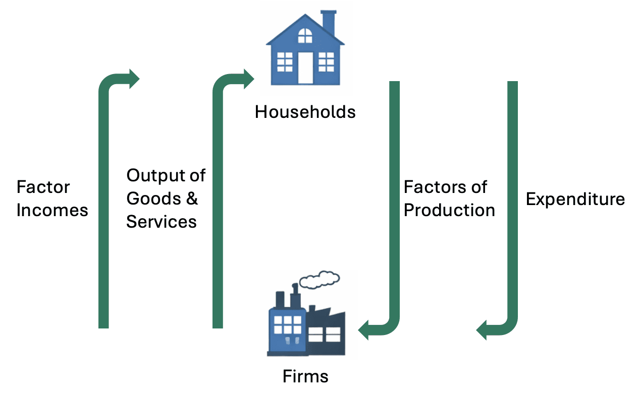
The diagram of the circular flow of income typically consists of two main boxes, one representing households and the other representing firms. Between these two boxes are arrows that show the flows. One set of arrows represents the flow of factor services from households to firms. These arrows usually move from households to firms and represent labour, land, capital, and enterprise being supplied to production.

A second set of arrows represents the flow of factor incomes from firms to households. These arrows move from firms to households and represent wages, rent, interest or dividends, and profit. This flow shows how households receive income by supplying factors of production.

A third set of arrows represents the flow of goods and services from firms to households. These arrows show the output produced by firms being supplied to households. Finally, a fourth set of arrows represents the flow of consumption expenditure from households to firms, showing households paying for the goods and services they consume.

An important implication of this model is that the value of output produced by firms is equal to the value of incomes earned by households. When firms produce goods and services, the value of that production is distributed to households in the form of factor incomes. There is no additional value created or lost in this process. Output and income are simply two ways of looking at the same economic activity.

At the same time, the value of output produced is also equal to the value of expenditure in the economy. This is because households spend all of their income on goods and services. Every unit of output produced by firms is purchased by households, and every unit of income earned by households is spent. As a result, total expenditure equals total output.

This leads to a key conclusion of the circular flow model. In this simplified economy, total income, total output, and total expenditure are equal. These are not three separate quantities but three different measures of the same level of economic activity. This identity lies at the heart of macroeconomic measurement and will later be used to define national income.

Because there are no leakages or injections in this model, it is described as a closed system. All income earned flows back into expenditure, and all expenditure generates income. There is no saving, no taxation, no government spending, and no international trade. While this does not reflect the complexity of a real economy, it provides a clear foundation for understanding how economic activity is generated.

The circular flow of income therefore serves two purposes. First, it explains how households and firms are mutually dependent. Firms rely on households for factor services, and households rely on firms for goods, services, and income. Second, it shows why income, output, and expenditure must be equal in aggregate. This equality is not the result of choice or intention but a consequence of the way the economic system is structured.

In the next stage of analysis, the assumptions of the closed system are relaxed. Households do not spend all of their income, governments collect taxes and spend money, and economies trade with the rest of the world. These features introduce leakages and injections into the circular flow, which alter the relationship between income, output, and expenditure.

Injections and Leakages within the Circular Flow

The simple circular flow of income model described earlier assumes that the economy operates as a closed system. In that model, households spend all of their income on goods and services produced by firms, and there is no government and no international trade. While this assumption is useful for introducing the basic relationships between income, output, and expenditure, it does not reflect how real economies function. In reality, money does not simply circulate endlessly between households and firms. Some income leaves the circular flow, and additional spending enters it from other sources.

These flows into and out of the circular flow are described using the concepts of injections and leakages. A leakage is a flow of income that removes spending power from the circular flow. An injection is a flow of expenditure that adds spending power to the circular flow. The presence of injections and leakages means that total expenditure in the economy is no longer equal to household consumption alone, and income is no longer automatically recycled back into spending.

There are three main leakages from the circular flow. The first leakage is saving by households. When households receive income in the form of wages, rent, interest or dividends, and profit, they do not necessarily spend all of this income on consumption. Some income may be set aside as saving. Saving represents income that is not used to purchase goods and services in the current period. As a result, saving withdraws spending from the circular flow, reducing the level of demand faced by firms.

The second leakage is taxation. Governments raise revenue by collecting taxes from households and firms. These taxes include direct taxes, such as income tax and corporation tax, and indirect taxes, such as value added tax and customs duties. When taxes are collected, income is removed from households and firms and does not immediately return to the circular flow as spending on goods and services. Taxation therefore represents a withdrawal of income from the circular flow.

The third leakage is spending on imports. When households, firms, or the government purchase goods and services produced in other countries, expenditure flows out of the domestic economy. This spending does not generate income for domestic firms and therefore does not support domestic production. Imports represent a leakage because money leaves the domestic circular flow and becomes income for producers abroad.

Alongside these leakages, there are three corresponding injections into the circular flow. The first injection is investment expenditure by firms. Investment refers to spending on capital goods that will be used in future production. These capital goods include machinery, factory buildings, transport equipment, and other productive assets. When firms invest, they create demand for goods and services in the current period, injecting additional spending into the circular flow. Investment is therefore an important source of expenditure that supports economic activity.

The second injection is government expenditure. Governments spend money on goods and services such as education, healthcare, infrastructure, and defence. This spending creates income for firms and households and adds to total demand in the economy. Government expenditure is an injection because it introduces spending into the circular flow that is not generated by household consumption.

The third injection is exports. Exports are goods and services produced in the domestic economy and sold to buyers in other countries. When foreign consumers or firms purchase domestic exports, money flows into the domestic economy from abroad. This expenditure creates income for domestic producers and represents an injection into the circular flow.

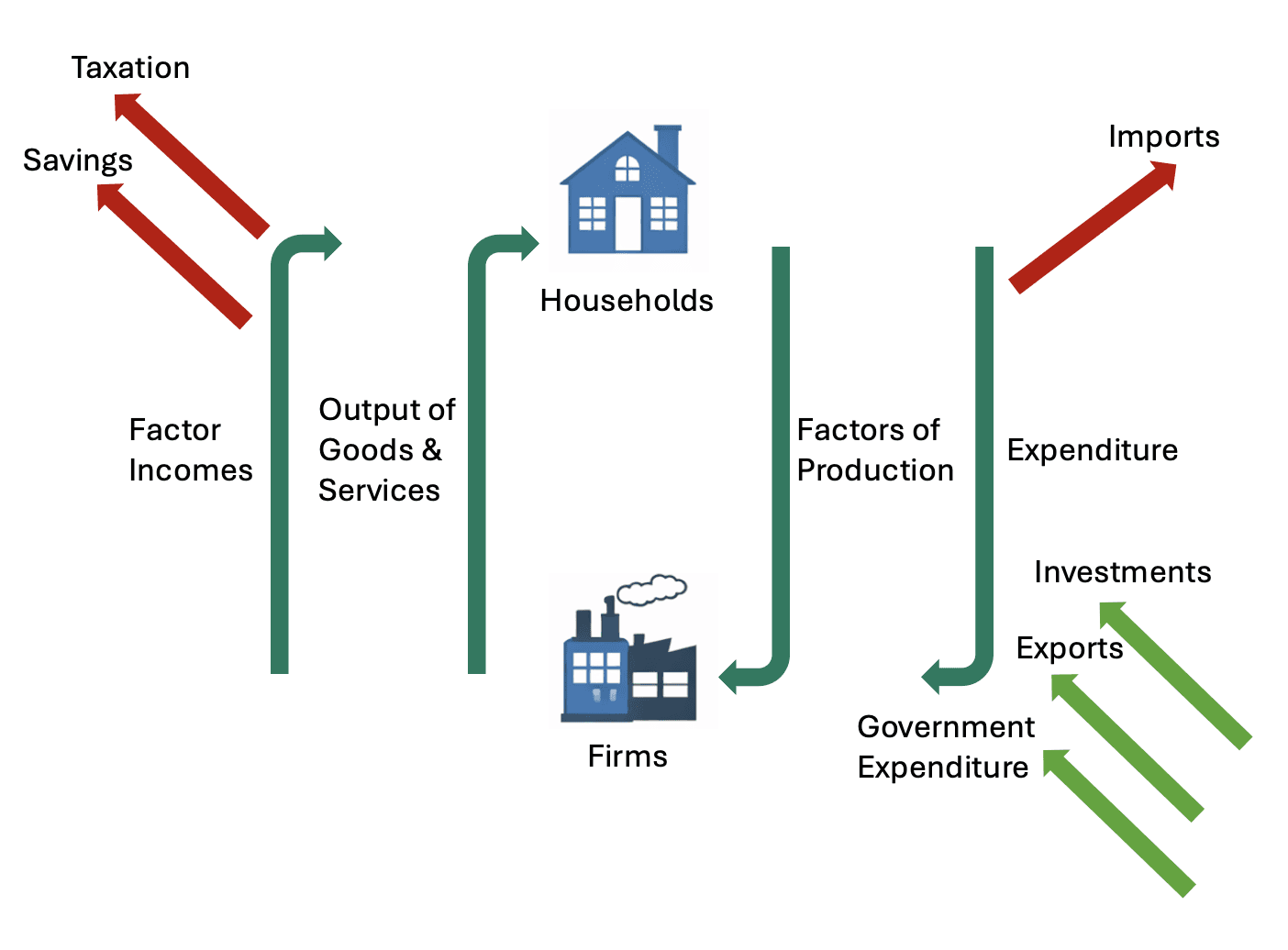
In the extended circular flow diagram, the basic flows between households and firms remain, but additional arrows are added to represent injections and leakages. Saving, taxation, and imports are shown as flows leaving the circular flow, while investment, government expenditure, and exports are shown as flows entering it. The presence of these flows means that total expenditure in the economy now consists of more than just household consumption.

Total expenditure is made up of consumption by households, investment by firms, government spending, and expenditure on exports. At the same time, some income is withdrawn through saving, taxation, and imports. The overall level of economic activity depends on the balance between these injections and leakages.

It is important to understand that injections and leakages are not necessarily equal at any point in time. If injections exceed leakages, total spending in the economy will rise. Firms will experience higher demand for their goods and services and are likely to increase production. This increase in production will require firms to hire more labour and use more factors of production, leading to higher incomes for households. The economy will expand as a result.

If leakages exceed injections, total spending in the economy will fall. Firms will face lower demand for their output and may reduce production. This reduction in production will lead to lower incomes for households, reinforcing the initial decline in spending. The economy will contract as a result.

The concepts of injections and leakages therefore provide a way of understanding how changes in saving behaviour, government policy, investment decisions, and international trade affect the level of economic activity. They also form the basis for analysing equilibrium in the overall economy, which is the subject of the next subchapter.

Balance in the Overall Economy

Once injections and leakages are introduced into the circular flow of income, the economy can no longer be described as a closed system. Income is no longer automatically recycled back into spending, and total expenditure is no longer determined solely by household consumption. Instead, the level of economic activity depends on the relationship between planned injections and planned leakages.

The economy is said to be in balance when planned injections are equal to planned leakages. Planned injections consist of investment expenditure by firms, government expenditure, and export expenditure. Planned leakages consist of household saving, taxation, and spending on imports. The term planned is important because it refers to the intended behaviour of economic agents rather than outcomes that occur by accident.

When planned injections equal planned leakages, total expenditure in the economy is just sufficient to purchase all of the goods and services that firms plan to produce. Firms are able to sell their output without accumulating unwanted stocks or running down existing inventories. In this situation, income, output, and expenditure remain stable over time.

To understand why this balance condition is important, consider what happens when injections exceed leakages. If firms plan to invest more, if the government increases its spending, or if exports rise, total planned expenditure in the economy increases. If households do not increase their saving, taxes do not rise, and imports do not increase by the same amount, injections will exceed leakages. As a result, total expenditure will be greater than the value of output firms had originally planned to produce.

Firms will then experience higher than expected demand for their goods and services. In response, they will increase production. To produce more output, firms will need to employ more labour and make greater use of other factors of production. This leads to an increase in factor incomes paid to households in the form of wages, rent, interest or dividends, and profit. As household incomes rise, consumption expenditure will also tend to increase, reinforcing the initial increase in demand. Through this process, the economy expands until a new balance is reached in which injections once again equal leakages.

Now consider the opposite case, where planned leakages exceed planned injections. If households decide to save a larger proportion of their income, if taxes rise, or if imports increase, income is withdrawn from the circular flow. If firms do not increase investment, if government spending does not rise, and if exports do not increase sufficiently to offset these withdrawals, total planned expenditure will fall.

Firms will then find that they are unable to sell all of the output they have produced. Stocks of unsold goods will begin to accumulate. In response, firms will reduce production. As production falls, firms will employ fewer factors of production, leading to lower incomes for households. With lower incomes, households will reduce their consumption expenditure, causing demand to fall further. This contractionary process will continue until a new balance is reached in which planned injections and planned leakages are equal at a lower level of income and output.

An important connection exists between saving and investment in this framework. When households save, their income is not spent on consumption goods. However, this saving does not disappear. Instead, it enters financial markets. Firms that wish to invest may borrow from these financial markets in order to finance their investment expenditure. In this way, household saving can be matched by firm investment, allowing leakages and injections to balance.

International trade also plays a role in determining balance in the overall economy. Part of the expenditure on goods and services in the economy may come from abroad in the form of export demand. At the same time, part of domestic expenditure may leak out of the economy through imports. Whether international trade adds to or subtracts from total demand depends on the relative sizes of exports and imports.

If export expenditure exceeds spending on imports, net exports are positive, and international trade contributes positively to injections. If imports exceed exports, net exports are negative, and international trade represents a net leakage from the circular flow.

The balance condition in the circular flow therefore provides a way of understanding how changes in behaviour and policy affect the level of economic activity. A change in saving habits, taxation, government spending, investment decisions, or international demand can all disturb the balance between injections and leakages. When this balance is disturbed, income, output, and employment adjust until a new balance is established.

This framework sets the foundation for measuring economic activity and for analysing how different components of spending contribute to total demand in the economy. The next step is to examine how national income, output, and expenditure are measured in practice.

Measuring National Income, Output and Expenditure

In macroeconomics, measuring the level of economic activity is essential for understanding how the economy is performing and how it changes over time. National income accounting provides a systematic way of measuring the total output produced by an economy, the total income earned within that economy, and the total expenditure on goods and services. These three measures are closely related and, under standard accounting conventions, are equal to one another.

The reason these three measures are equal lies in the structure of the circular flow of income. Every good or service that is produced generates income for the factors of production involved. At the same time, every unit of income earned is either spent or saved, and expenditure on goods and services represents the purchase of output. As a result, output, income, and expenditure are not separate concepts but different perspectives on the same underlying level of economic activity.

There are three main methods used to measure national income. These are the output method, the income method, and the expenditure method. Each method measures economic activity in a different way, but when calculated correctly, all three methods produce the same total value.

The output method measures national income by calculating the total value of goods and services produced within the economy over a given period of time. This involves adding together the value added at each stage of production. Value added refers to the increase in value that occurs when a firm uses inputs to produce an output. It is calculated as the value of a firm’s output minus the value of intermediate goods used up in the production process.

The concept of value added is essential to avoid double counting. Double counting occurs when the value of intermediate goods is included multiple times in the calculation of total output. For example, if the value of raw materials, components, and final goods were all added together, the same value would be counted more than once. By focusing on value added at each stage, the output method ensures that only the final value of production is included in national income.

The income method measures national income by adding together all the incomes earned by the factors of production in the economy. These factor incomes arise directly from the production process. Labour earns wages and salaries. Land earns rent. Capital earns interest or dividends. Enterprise earns profit. By summing all of these incomes, the income method captures the total value generated by production.

In practice, the income method may also include adjustments for items such as indirect taxes and subsidies. Indirect taxes raise the market price of goods and services above the income received by producers, while subsidies lower the market price below the income received by producers. These adjustments ensure that the income measure corresponds to the value of output measured at market prices.

The expenditure method measures national income by adding together all spending on final goods and services within the economy over a given period of time. Expenditure on intermediate goods is excluded, since these goods are used up in the production of final goods and services. Including them would again result in double counting.

Using the expenditure method, total expenditure in the economy is divided into several broad categories. Household consumption refers to spending by households on goods and services, such as food, clothing, and transport. Investment refers to spending by firms on capital goods that will be used in future production, such as machinery, buildings, and equipment. Government expenditure refers to spending by the government on goods and services, such as education, healthcare, and infrastructure. Export expenditure refers to spending by foreign buyers on domestically produced goods and services.

Spending on imports is not included in national income because imports represent expenditure on goods and services produced outside the domestic economy. While imports are included in consumption, investment, or government spending figures, they must be subtracted to avoid overstating domestic production. This leads to the concept of net exports, which is defined as exports minus imports.

The equality of the three methods can be understood by returning to the circular flow of income. The value of output produced by firms generates incomes for households in the form of wages, rent, interest or dividends, and profit. These incomes are then used to finance expenditure on goods and services. As a result, output gives rise to income, and income gives rise to expenditure. Measuring any one of these flows captures the same underlying economic activity.

It is important to recognise that national income measures record flows rather than stocks. A flow is a quantity measured over a period of time, such as one year. National income measures the value of output produced over a given period, not the total wealth accumulated at a point in time. This distinction is essential for interpreting national income statistics correctly.

National income figures are used for a variety of purposes. They allow economists to compare the performance of an economy over time, to compare the size of different economies, and to assess the impact of economic policies. However, these measures also have limitations, which will be explored later in the chapter.

The measurement of national income provides the foundation for understanding aggregate demand. Once total expenditure is broken down into its components, it becomes possible to analyse how changes in consumption, investment, government spending, and net exports affect the overall level of demand in the economy. This analysis begins by examining the concept of gross domestic product, which is the most widely used measure of national output.

Gross Domestic Product and Real GDP

Gross domestic product is the most commonly used measure of national output. It measures the total value of all final goods and services produced within the domestic economy over a given period of time, usually one year. The word domestic is important because it refers only to production that takes place within the geographical boundaries of the economy, regardless of who owns the factors of production. The word final is also important because it ensures that intermediate goods are excluded in order to avoid double counting.

Gross domestic product is a flow measure. It records production that occurs over a period of time rather than measuring the total stock of goods or wealth at a single point in time. This means that gross domestic product captures the level of current economic activity rather than accumulated economic resources.

When gross domestic product is measured using the expenditure method, it is calculated by adding together all spending on final goods and services produced within the economy. This includes household consumption expenditure, investment expenditure by firms, government expenditure on goods and services, and export expenditure. From this total, expenditure on imports is subtracted, since imports represent spending on goods and services produced outside the domestic economy. The result is total expenditure on domestically produced output.

Gross domestic product can also be measured using the output method and the income method, as discussed earlier. Regardless of the method used, the final figure for gross domestic product should be the same, since all three methods measure the same underlying level of economic activity from different perspectives.

An important distinction must be made between nominal gross domestic product and real gross domestic product. Nominal gross domestic product measures the value of output using current prices in the year in which the output is produced. This means that changes in nominal gross domestic product can result from changes in the quantity of output, changes in prices, or both.

For example, if nominal gross domestic product increases from one year to the next, this does not necessarily mean that the economy is producing more goods and services. The increase could be due entirely to higher prices, with no change in the physical volume of output. As a result, nominal gross domestic product is not a reliable measure of changes in real economic activity over time.

Real gross domestic product addresses this problem by adjusting for changes in the price level. Real gross domestic product measures the value of output using constant prices from a chosen base year. By holding prices constant, real gross domestic product isolates changes in the quantity of goods and services produced. This allows meaningful comparisons of economic output over time.

The process of converting nominal gross domestic product into real gross domestic product involves removing the effects of inflation. Inflation refers to a sustained increase in the overall price level in the economy. When inflation occurs, nominal values rise even if the underlying quantities remain unchanged. By adjusting for inflation, real gross domestic product reflects only changes in real production.

The relationship between nominal and real gross domestic product can be explained step by step. Nominal gross domestic product is calculated by multiplying quantities of goods and services produced by their current prices and summing the results. Real gross domestic product is calculated by multiplying the same quantities by base year prices instead. The difference between the two measures captures the effect of price changes over time.

Real gross domestic product is therefore a more accurate indicator of changes in living standards and economic growth. When real gross domestic product increases, the economy is producing a larger quantity of goods and services. This generally allows for higher consumption, greater investment, and improved material well being, although real gross domestic product does not capture all aspects of economic welfare.

Gross domestic product also differs from other measures of national income that may appear in broader macroeconomic analysis. For example, gross domestic product focuses on production within the domestic economy, while other measures may focus on income earned by residents regardless of where production takes place. In this chapter, the emphasis remains on gross domestic product because it provides the most direct link to aggregate demand and total spending.

Despite its widespread use, gross domestic product has limitations as a measure of economic performance. It does not account for income distribution, unpaid work, environmental costs, or differences in leisure time. However, within the framework of macroeconomic analysis, gross domestic product remains a central concept because it provides a consistent and measurable indicator of economic activity.

Understanding the distinction between nominal and real gross domestic product is essential before moving on to aggregate demand. Aggregate demand is concerned with total spending in the economy, and changes in aggregate demand affect real output rather than nominal values alone. The next step is therefore to examine the components of aggregate demand in detail.

The Components of Aggregate Demand

Aggregate demand refers to the total level of planned expenditure on goods and services in an economy over a given period of time. It represents the demand for the economy’s output as a whole rather than demand in any single market. Aggregate demand is a central concept in macroeconomics because it determines the overall level of economic activity and therefore influences output, income, and employment.

Aggregate demand is made up of several distinct components, each corresponding to a different source of spending in the economy. These components arise directly from the extended circular flow of income, where expenditure comes not only from households but also from firms, government, and the rest of the world. By separating aggregate demand into its components, it becomes possible to analyse how changes in different types of spending affect total demand and economic performance.

The first component of aggregate demand is consumption. Consumption refers to spending by households on goods and services. This includes expenditure on items such as food, clothing, housing services, transport, and leisure services. Consumption is typically the largest component of aggregate demand in most economies. It is closely linked to household income, since households use their income earned from wages, rent, interest or dividends, and profit to finance their spending.

Consumption spending plays a key role in sustaining economic activity. When households spend more, firms experience higher demand for their output. In response, firms increase production, which leads to higher employment and incomes. These higher incomes then support further consumption spending, reinforcing the initial increase in demand. Conversely, when households reduce consumption, firms face lower demand, leading to reductions in output and income.

The second component of aggregate demand is investment. Investment refers to spending by firms on capital goods that are used to produce other goods and services in the future. These capital goods include machinery, equipment, factories, offices, and infrastructure. Investment is distinct from consumption because it is not undertaken to satisfy current wants directly but to increase future productive capacity.

Investment expenditure is often more volatile than consumption expenditure. Firms make investment decisions based on expectations about future demand, costs, and profitability. If firms are optimistic about future economic conditions, they are more likely to invest in new capital. If they are pessimistic, they may postpone or cancel investment projects. As a result, changes in investment can lead to significant fluctuations in aggregate demand.

The third component of aggregate demand is government expenditure. Government expenditure refers to spending by the government on goods and services. This includes spending on public sector wages, education, healthcare, defence, transport infrastructure, and other public services. Government expenditure contributes directly to aggregate demand because it represents spending on current output.

It is important to distinguish government expenditure from transfer payments. Transfer payments, such as pensions or unemployment benefits, do not represent spending on goods and services. Instead, they involve the redistribution of income from one group to another. While transfer payments may indirectly affect consumption, they are not included directly as a component of aggregate demand.

Government expenditure can play an important role in stabilising the economy. Changes in government spending can increase or decrease aggregate demand independently of household and firm behaviour. For this reason, government expenditure is often a key policy tool in macroeconomic management.

The fourth component of aggregate demand is net exports. Net exports are defined as exports minus imports. Exports are goods and services produced domestically and sold to buyers in other countries. Export expenditure represents spending that flows into the domestic economy from abroad and therefore adds to aggregate demand.

Imports are goods and services produced abroad and purchased by domestic households, firms, or the government. Spending on imports does not generate demand for domestically produced output. As a result, imports must be subtracted when calculating aggregate demand to avoid overstating the demand for domestic production.

Net exports can be positive or negative. If export expenditure exceeds import expenditure, net exports are positive and contribute positively to aggregate demand. If import expenditure exceeds export expenditure, net exports are negative and reduce aggregate demand.

By combining these four components, aggregate demand can be expressed as total spending on domestically produced goods and services. Consumption, investment, government expenditure, and net exports together represent all sources of demand for output in the economy.

Understanding the components of aggregate demand is essential because each component responds to different influences. Consumption is closely related to income and household confidence. Investment depends heavily on expectations and profitability. Government expenditure reflects policy decisions. Net exports depend on conditions in the global economy and relative competitiveness. Changes in any one component can therefore shift aggregate demand and alter the level of economic activity.

Consumption and Income

Consumption is the largest component of aggregate demand in most economies, and understanding what determines consumption is essential for explaining changes in overall economic activity. At the macroeconomic level, consumption refers to total spending by households on goods and services over a given period of time. While individual households differ in their spending patterns, macroeconomic analysis focuses on the relationship between total consumption and total income across the economy.

A central idea in macroeconomics is that consumption is positively related to income. This means that, in general, as household income rises, consumption increases, and as household income falls, consumption decreases. This relationship exists because income provides households with the ability to spend. Without income, consumption is constrained.

To understand this relationship clearly, it is useful to distinguish between income and consumption as aggregate variables. Aggregate income refers to the total income earned by all households in the economy. This income is generated through the circular flow of income as households receive wages, rent, interest or dividends, and profit in exchange for supplying factors of production. Aggregate consumption refers to the total spending by households on goods and services.

The relationship between consumption and income can be represented using a consumption function. A consumption function shows how the level of consumption depends on the level of income. In its simplest form, the consumption function assumes a stable and predictable relationship between income and consumption across the economy.

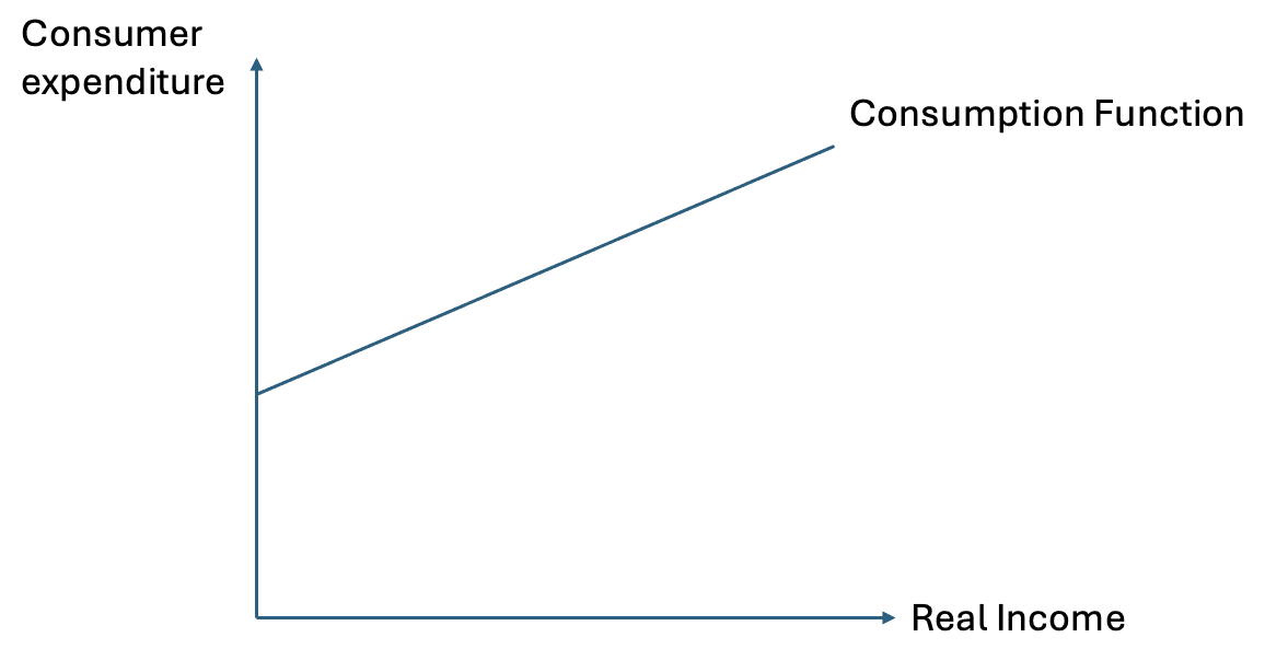
In the consumption function diagram, income is measured on the horizontal axis and consumption is measured on the vertical axis. The consumption function is shown as an upward sloping line. The positive slope of the line reflects the fact that as income increases, consumption also increases. However, the slope is less than one, meaning that consumption rises by less than the full increase in income.

This feature of the consumption function reflects the idea that households do not spend all of any increase in income. When income rises, households typically increase both consumption and saving. As a result, consumption increases, but by a smaller amount than the increase in income.

An important concept associated with the consumption function is autonomous consumption. Autonomous consumption refers to the level of consumption that occurs even when income is zero. This consumption is financed through past savings, borrowing, or transfers. On the diagram, autonomous consumption is represented by the point where the consumption function intersects the vertical axis. This intercept shows that households may still consume some goods and services even if current income is very low.

Another key concept is induced consumption. Induced consumption refers to the portion of consumption that depends directly on income. As income rises, induced consumption increases. The slope of the consumption function captures how responsive consumption is to changes in income.

The marginal propensity to consume is a measure of this responsiveness. The marginal propensity to consume is defined as the proportion of an additional unit of income that is spent on consumption. For example, if households spend 0.8 of each additional unit of income on consumption, the marginal propensity to consume is 0.8. The marginal propensity to consume determines the steepness of the consumption function. A higher marginal propensity to consume results in a steeper consumption function, while a lower marginal propensity to consume results in a flatter one.

Because households do not spend all of their income, saving plays an important role alongside consumption. Saving is defined as income that is not spent on consumption. At the macroeconomic level, saving represents a leakage from the circular flow of income. As income increases, saving also increases, because households allocate part of their additional income to saving.

The relationship between consumption and income therefore has important implications for aggregate demand. When income rises, consumption rises, increasing aggregate demand. When income falls, consumption falls, reducing aggregate demand. This creates a feedback effect in the economy. Changes in income affect consumption, and changes in consumption affect income through changes in firms’ production and employment decisions.

The stability of the consumption income relationship is crucial for macroeconomic analysis. If households behaved unpredictably, it would be difficult to analyse or manage aggregate demand. The assumption that consumption depends primarily on income allows economists to explain why changes in investment, government spending, or exports can have amplified effects on total output through their impact on income and consumption.

Understanding consumption and income also prepares the ground for analysing other influences on consumption. While income is the most important determinant, it is not the only factor that affects how much households choose to spend.

Other Influences on Consumption

While income is the primary determinant of consumption at the macroeconomic level, it is not the only factor that influences how much households choose to spend. Even when income remains unchanged, consumption can rise or fall due to changes in other conditions that affect household decision making. These influences help explain why consumption does not always move in perfect proportion with income and why aggregate demand can change even when income is stable.

One important influence on consumption is household wealth. Wealth refers to the stock of assets owned by households, such as savings, property, and financial investments. Unlike income, which is a flow measured over time, wealth is a stock measured at a point in time. When household wealth increases, households may feel more financially secure and therefore more willing to spend a higher proportion of their income. This can lead to an increase in consumption even if current income has not changed. Conversely, a fall in wealth can cause households to reduce consumption in order to rebuild their asset holdings.

Another key influence on consumption is the availability of credit. Credit allows households to spend more than their current income by borrowing. When credit is easily available and borrowing conditions are favourable, households may increase consumption, particularly on durable goods such as cars and household equipment. Easier access to credit reduces the need to postpone consumption until sufficient income has been earned. When credit conditions tighten, borrowing becomes more difficult or more expensive, and households may reduce consumption, even if their income remains unchanged.

Interest rates also influence consumption decisions. Interest rates represent the cost of borrowing and the reward for saving. When interest rates are low, borrowing becomes cheaper, encouraging households to finance consumption through credit. At the same time, the return on saving is reduced, which may make saving less attractive relative to spending. As a result, lower interest rates tend to encourage higher consumption. When interest rates are high, borrowing is more expensive and saving becomes more attractive, which can lead households to reduce consumption.

Expectations about future income play an important role in shaping consumption behaviour. Households do not base their spending decisions solely on their current income. Instead, they consider their expected future income. If households expect their income to rise in the future, they may be willing to increase consumption in the present, even if current income is unchanged. If households expect their income to fall or become less secure, they may reduce consumption and increase saving as a precaution.

Expectations about future economic conditions more broadly also affect consumption. If households are confident about the state of the economy and expect stable employment and rising incomes, they are more likely to spend. If households are pessimistic about economic prospects, concerned about unemployment, or uncertain about future conditions, they may cut back on consumption. This behaviour reflects precautionary saving, where households save more to protect themselves against possible future income losses.

Changes in taxation can also influence consumption. A reduction in taxes increases households’ disposable income, which is the income available to spend or save after taxes have been paid. An increase in disposable income tends to raise consumption, although the size of the increase depends on the marginal propensity to consume. Conversely, an increase in taxes reduces disposable income and can lead to a fall in consumption.

Demographic factors may also affect aggregate consumption. Changes in the age structure of the population can influence spending patterns. For example, a population with a larger proportion of working age households may have higher consumption than a population with a larger proportion of retirees, even if average income levels are similar. While demographic changes tend to occur slowly, they can have long run effects on consumption and aggregate demand.

All of these influences affect consumption by shifting the consumption function. When households become more willing to spend at each level of income, the consumption function shifts upward. When households become more cautious and reduce spending at each level of income, the consumption function shifts downward. These shifts alter aggregate demand independently of changes in income.

Understanding these additional influences on consumption is important because they help explain why consumption can change suddenly or unexpectedly. A loss of confidence, a tightening of credit conditions, or a fall in wealth can all reduce consumption and weaken aggregate demand, even if income has not yet fallen. Similarly, rising confidence, easier credit, or tax cuts can stimulate consumption and strengthen aggregate demand.

With consumption fully analysed, attention can now turn to the next component of aggregate demand, investment. Investment behaves very differently from consumption and is influenced by a distinct set of factors.

Investment

Investment is a key component of aggregate demand and plays a central role in determining the level of economic activity in the economy. In macroeconomics, investment has a specific meaning that differs from its everyday use. Investment refers to spending by firms on capital goods that are used to produce other goods and services in the future. These capital goods include machinery, equipment, factories, offices, and infrastructure.

Investment does not include the purchase of financial assets such as shares or bonds. Buying shares represents a transfer of ownership of existing assets rather than the creation of new productive capacity. In macroeconomic analysis, only spending that adds to the economy’s stock of capital goods is classified as investment.

Investment is important for two reasons. First, it is a component of aggregate demand and therefore affects current economic activity. When firms invest, they create demand for goods and services such as construction, machinery, and professional services. This demand generates income for households and contributes to overall spending in the economy. Second, investment increases the economy’s productive capacity by expanding or improving the capital stock. This affects the economy’s ability to produce goods and services in the future.

Investment spending is typically more volatile than consumption spending. Firms make investment decisions based on expectations about future demand, costs, and profitability. Because these expectations can change rapidly, investment can rise or fall sharply over short periods of time, making it a major source of economic fluctuations.

One of the most important influences on investment is the expected profitability of investment projects. Firms compare the expected revenue generated by an investment with the costs involved in undertaking it. If firms expect demand for their products to rise in the future, they are more likely to invest in new capital to expand production. If demand is expected to fall or remain weak, firms may delay or cancel investment plans.

Interest rates also influence investment decisions. Interest rates represent the cost of borrowing funds to finance investment and the opportunity cost of using internal funds. When interest rates are low, borrowing is cheaper and investment projects are more likely to be profitable. As a result, lower interest rates tend to encourage higher levels of investment. When interest rates are high, borrowing becomes more expensive and fewer investment projects are profitable, leading to lower investment.

Business confidence and expectations about the future state of the economy play a crucial role in determining investment. Even if interest rates are low, firms may be reluctant to invest if they are uncertain about future economic conditions. Political uncertainty, economic instability, or weak consumer demand can all reduce business confidence and lead to lower investment spending.

Technological change can also affect investment. The introduction of new technologies may create opportunities for firms to improve productivity or reduce costs. In response, firms may invest in new machinery or equipment to adopt these technologies. Conversely, periods of slow technological progress may be associated with lower investment.

Investment is also influenced by government policy. Tax policies that affect corporate profits, investment allowances, or depreciation can alter the cost and attractiveness of investment. Government spending on infrastructure can also encourage private investment by improving the environment in which firms operate.

Because investment is both a component of aggregate demand and a determinant of future productive capacity, changes in investment have both short run and long run effects on the economy. A fall in investment reduces current aggregate demand and can lead to lower output and employment. At the same time, it slows the growth of the capital stock, which may reduce future output.

Government Expenditure

Government expenditure is an important component of aggregate demand and represents spending by the public sector on goods and services. In macroeconomic analysis, government expenditure refers specifically to spending that directly contributes to current production and income in the economy. This includes spending on public services, infrastructure, and the wages of public sector workers.

Government expenditure must be clearly distinguished from government transfers. Transfer payments, such as pensions, unemployment benefits, or income support, involve the redistribution of income from one group to another rather than the purchase of goods and services. While transfer payments may indirectly affect consumption by altering household income, they do not represent direct spending on output and are therefore not included as a component of aggregate demand.

Government expenditure enters the circular flow of income as an injection. When the government purchases goods and services, it creates demand for output produced by firms. This demand generates income for households in the form of wages, rent, interest or dividends, and profit. As a result, government expenditure directly increases aggregate demand and supports economic activity.

One key feature of government expenditure is that it is determined largely by policy decisions rather than by income. Unlike consumption, which depends primarily on household income, government spending is set through political and budgetary processes. This means that government expenditure can change independently of current economic conditions.

Because government expenditure does not depend directly on income, it can play a stabilising role in the economy. During periods of economic downturn, governments may increase spending in order to support demand and reduce unemployment. During periods of strong economic growth, governments may reduce spending or allow it to grow more slowly in order to prevent excessive demand.

Government spending takes many forms. Expenditure on education and healthcare provides services directly to households while also employing large numbers of workers. Spending on infrastructure, such as roads, transport systems, and public buildings, supports both current demand and future productive capacity. Defence and public administration also represent significant areas of government expenditure in many economies.

The impact of government expenditure on aggregate demand depends on its size and composition. An increase in government spending directly increases total expenditure in the economy. Firms receiving government contracts increase production to meet this demand, leading to higher employment and incomes. These higher incomes may then support additional consumption spending, reinforcing the initial increase in demand.

Government expenditure is financed through taxation, borrowing, or a combination of both. When spending is financed through taxation, the increase in government expenditure may be partially offset by a reduction in household or firm spending due to higher taxes. When spending is financed through borrowing, the immediate impact on aggregate demand may be larger, since taxation does not rise at the same time.

The relationship between government expenditure and aggregate demand highlights the role of the public sector in influencing economic outcomes. By adjusting its level of spending, the government can affect total demand, output, and employment in the economy. This makes government expenditure a central tool in macroeconomic policy.

Net Exports

Net exports are the final component of aggregate demand and capture the role of international trade in determining the level of demand for domestically produced output. Net exports are defined as the value of exports minus the value of imports over a given period of time. They can be positive, negative, or zero, depending on the relative size of exports and imports.

Exports are goods and services that are produced within the domestic economy and sold to buyers in other countries. When foreign households, firms, or governments purchase domestically produced output, expenditure flows into the domestic economy from abroad. This spending creates income for domestic firms and households and therefore represents an injection into the circular flow of income. Export expenditure adds directly to aggregate demand because it increases demand for domestically produced goods and services.

Imports are goods and services that are produced in other countries and purchased by domestic households, firms, or the government. When imports are purchased, expenditure flows out of the domestic economy and becomes income for producers abroad. Spending on imports does not create demand for domestic output and therefore represents a leakage from the circular flow of income.

Because consumption, investment, and government expenditure may all include spending on imported goods and services, imports must be subtracted when calculating aggregate demand. If imports were not subtracted, total spending on domestic output would be overstated, since part of that spending would be directed toward foreign production.

Net exports combine these two flows into a single measure. When export expenditure exceeds import expenditure, net exports are positive. In this case, international trade adds to aggregate demand and increases the level of economic activity. When import expenditure exceeds export expenditure, net exports are negative. In this case, international trade reduces aggregate demand and acts as a net leakage from the circular flow.

Net exports depend on several factors. One important factor is the level of income in the domestic economy. As domestic income rises, households and firms tend to increase their spending, including spending on imported goods and services. This causes imports to rise. As a result, higher domestic income can lead to a deterioration in net exports if exports do not increase at the same time.

The level of income in other countries also affects net exports. When foreign economies grow and incomes abroad rise, foreign demand for domestically produced goods and services tends to increase. This leads to higher exports and an improvement in net exports. When foreign economies experience downturns, export demand may fall, reducing net exports.

Relative prices between countries influence net exports as well. If domestically produced goods become relatively cheaper compared to foreign goods, exports may rise and imports may fall, improving net exports. If domestic goods become relatively more expensive, exports may fall and imports may rise, worsening net exports.

Exchange rates play a key role in determining relative prices in international trade. An appreciation of the domestic currency makes exports more expensive for foreign buyers and imports cheaper for domestic consumers. This tends to reduce exports and increase imports, worsening net exports. A depreciation of the domestic currency makes exports cheaper for foreign buyers and imports more expensive for domestic consumers, which tends to improve net exports.

Net exports therefore connect the domestic economy to the global economy. Changes in global economic conditions, exchange rates, and relative competitiveness can all affect aggregate demand through their impact on exports and imports. Because these factors are often outside the control of domestic households and firms, net exports can be a source of external shocks to the economy.

The inclusion of net exports completes the breakdown of aggregate demand into its four components. Aggregate demand is now understood as total planned expenditure on domestically produced goods and services coming from households, firms, the government, and foreign buyers.

The Importance of Expectations

Expectations play a central role in macroeconomics because many economic decisions are based not only on current conditions but also on beliefs about the future. Households, firms, and governments all form expectations about future income, prices, demand, and economic stability, and these expectations influence their current spending behaviour. As a result, expectations can affect aggregate demand even when current income and prices have not changed.

For households, expectations about future income are particularly important for consumption decisions. When households expect their income to rise in the future, they may feel confident that they will be able to maintain or increase their standard of living. This confidence can lead them to increase consumption in the present, even if their current income remains unchanged. Conversely, if households expect their future income to fall or become uncertain, they may reduce consumption and increase saving as a precaution.

Expectations about future prices also influence household behaviour. If households expect prices to rise in the future, they may bring forward consumption in order to purchase goods and services before prices increase. This increases current consumption and raises aggregate demand. If households expect prices to fall, they may delay consumption, reducing current aggregate demand.

Firms are also strongly influenced by expectations, particularly in relation to investment decisions. Investment involves committing resources in the present in order to produce goods and services in the future. As a result, firms base investment decisions on their expectations of future demand, costs, and profitability. If firms expect demand for their products to increase, they are more likely to invest in new capital to expand production. If they expect demand to weaken, they may reduce or postpone investment spending.

Expectations about future costs, including wages, interest rates, and taxes, also affect investment decisions. If firms expect interest rates to rise, borrowing costs may increase in the future, making current investment more attractive. If firms expect higher taxes or higher wage costs, this may reduce expected profitability and discourage investment.

Expectations play a role in government decision making as well. Governments may adjust their spending and taxation policies based on expectations about future economic conditions. For example, if the government expects an economic downturn, it may increase spending in order to support demand. If it expects the economy to overheat, it may reduce spending or increase taxes to limit demand.

In the context of international trade, expectations about exchange rates and foreign economic conditions influence export and import decisions. If firms expect the domestic currency to depreciate in the future, they may increase export activity in anticipation of higher foreign demand. If households expect imported goods to become more expensive, they may reduce import spending or bring forward purchases.

The importance of expectations means that aggregate demand can change suddenly and without any immediate change in income, prices, or policy. A shift in confidence or sentiment can alter spending decisions across the economy. For example, a loss of consumer confidence can reduce consumption, while a loss of business confidence can reduce investment. These changes in spending directly affect aggregate demand.

Expectations can also create self reinforcing effects. If households and firms become pessimistic about the future, they may reduce spending. This reduction in spending lowers aggregate demand, leading to lower output and income. Lower income then reinforces pessimism, further reducing spending. Similarly, optimism can lead to increased spending, higher output, and rising incomes, reinforcing positive expectations.

Because expectations are based on beliefs rather than certainties, they introduce an element of instability into the economy. Changes in expectations can amplify economic fluctuations and make it more difficult to predict economic outcomes. For this reason, managing expectations is often an important part of economic policy.

The Aggregate Demand Curve

The aggregate demand curve is a graphical representation of the relationship between the overall price level in the economy and the total quantity of goods and services demanded over a given period of time. It brings together all components of aggregate demand and shows how total planned expenditure changes as the price level changes, holding all other influences constant.

Aggregate demand is concerned with total spending on domestically produced output. This includes consumption by households, investment by firms, government expenditure, and net exports. The aggregate demand curve therefore reflects the combined spending decisions of households, firms, government, and foreign buyers at different price levels.

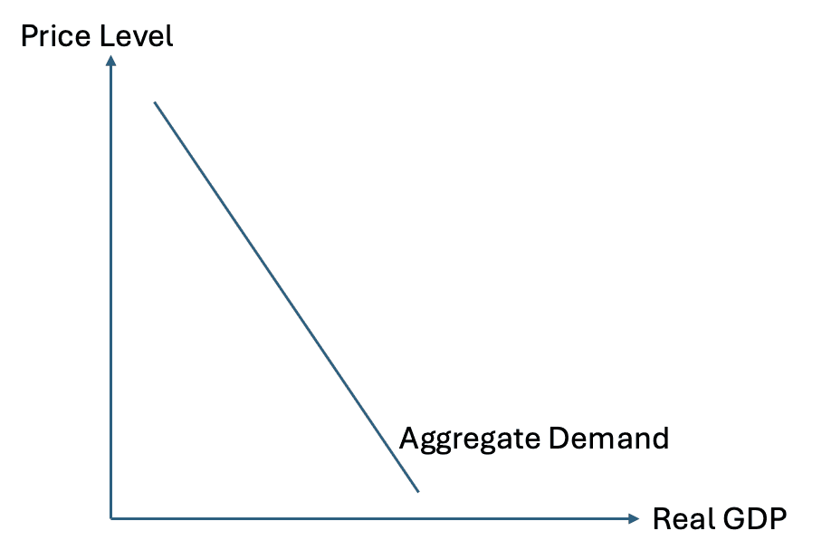
In the aggregate demand diagram, the vertical axis measures the overall price level. This is not the price of a single good but an index that reflects the average level of prices across the entire economy. The horizontal axis measures real output, which represents the total quantity of goods and services produced in the economy, measured in real terms using constant prices.

The aggregate demand curve slopes downward from left to right. This downward slope indicates that, as the overall price level falls, the quantity of goods and services demanded increases, and as the overall price level rises, the quantity of goods and services demanded decreases. This relationship is a central feature of aggregate demand and must be understood carefully.

One reason for the downward slope of the aggregate demand curve is the effect of the price level on consumption. When the overall price level falls, the purchasing power of household income increases. With greater purchasing power, households are able to buy more goods and services with the same nominal income, leading to higher consumption expenditure. When the price level rises, purchasing power falls, reducing consumption.

A second reason for the downward slope involves investment. When the price level falls, interest rates may also fall. Lower interest rates reduce the cost of borrowing, making more investment projects profitable. As a result, firms increase investment spending, raising aggregate demand. When the price level rises, interest rates may rise, discouraging investment and reducing aggregate demand.

A third reason for the downward slope relates to net exports. When the domestic price level falls relative to price levels in other countries, domestically produced goods become more competitive in international markets. Exports tend to increase, and imports may decrease, improving net exports. This increase in net exports raises aggregate demand. When the domestic price level rises, exports become less competitive and imports more attractive, reducing net exports and lowering aggregate demand.

Each point on the aggregate demand curve represents a situation in which total planned expenditure on domestically produced goods and services is equal to the level of output demanded at that price level. Movements along the aggregate demand curve occur when there is a change in the overall price level, causing a change in the quantity of output demanded.

It is important to distinguish between the aggregate demand curve and individual market demand curves. While individual demand curves show the relationship between price and quantity demanded for a specific good, the aggregate demand curve shows the relationship between the overall price level and total output demanded across the entire economy. The downward slope of aggregate demand arises from macroeconomic mechanisms rather than substitution effects between goods.

The aggregate demand curve provides a framework for analysing how changes in prices affect total spending and output. However, changes in factors other than the price level can also affect aggregate demand. These changes do not cause movements along the aggregate demand curve but instead shift the entire curve. Understanding these shifts is essential for explaining changes in economic activity.

Movements Along and Shifts of the Aggregate Demand Curve

Understanding aggregate demand requires a clear distinction between movements along the aggregate demand curve and shifts of the aggregate demand curve. Although both involve changes in the quantity of output demanded, they arise from different causes and have different economic meanings. Confusing these two concepts leads to fundamental errors in macroeconomic analysis, so the distinction must be made explicit.

A movement along the aggregate demand curve occurs when there is a change in the overall price level, with all other determinants of aggregate demand held constant. In this case, the aggregate demand curve itself does not change position. Instead, the economy moves from one point to another along the same curve.

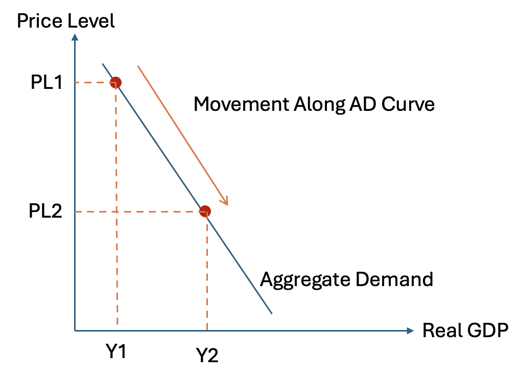
In the diagram, the vertical axis shows the overall price level, and the horizontal axis shows real output. The aggregate demand curve slopes downward from left to right. Suppose the economy initially operates at a point on the aggregate demand curve where the price level is relatively high. If the overall price level falls, there is a movement down the aggregate demand curve to the right, indicating an increase in the quantity of goods and services demanded.

This movement occurs because a lower price level increases the purchasing power of income, encourages higher consumption, reduces interest rates and stimulates investment, and improves the competitiveness of exports relative to imports. All of these effects raise total planned expenditure, increasing the quantity of output demanded. The key point is that the only change causing this movement is a change in the overall price level.

Conversely, if the overall price level rises, there is a movement up the aggregate demand curve to the left. Higher prices reduce purchasing power, discourage consumption, raise interest rates and reduce investment, and worsen net exports. These effects reduce total planned expenditure, lowering the quantity of output demanded. Again, the aggregate demand curve itself does not move.

A shift of the aggregate demand curve occurs when there is a change in any factor other than the overall price level that affects total planned expenditure. When aggregate demand shifts, the entire curve moves either to the right or to the left. A rightward shift indicates an increase in aggregate demand at every price level, while a leftward shift indicates a decrease in aggregate demand at every price level.

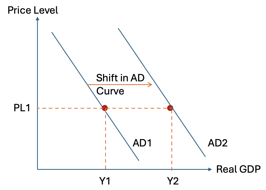
A rightward shift of the aggregate demand curve occurs when one or more components of aggregate demand increase. An increase in consumption due to higher income, greater confidence, lower taxes, or increased wealth will raise aggregate demand. An increase in investment due to higher business confidence, technological change, or lower interest rates will also raise aggregate demand. An increase in government expenditure directly raises aggregate demand. An increase in net exports due to higher foreign income or improved competitiveness also raises aggregate demand.

When aggregate demand shifts to the right, at every possible price level the quantity of goods and services demanded is higher than before. This reflects an increase in total planned expenditure across the economy.

A leftward shift of the aggregate demand curve occurs when one or more components of aggregate demand decrease. A fall in consumption due to lower income, reduced confidence, higher taxes, or falling wealth reduces aggregate demand. A fall in investment due to pessimistic expectations or higher interest rates reduces aggregate demand. A reduction in government expenditure lowers aggregate demand. A fall in net exports due to weaker foreign demand or rising imports also reduces aggregate demand.

When aggregate demand shifts to the left, at every possible price level the quantity of goods and services demanded is lower than before. This reflects a decrease in total planned expenditure across the economy.

It is essential to emphasise that changes in the price level do not shift the aggregate demand curve. Changes in the price level only cause movements along the curve. Shifts occur only when there is a change in consumption, investment, government expenditure, or net exports that is independent of the price level.

This distinction allows macroeconomists to analyse different types of economic change. Inflation or deflation involves movements along the aggregate demand curve. Changes in confidence, policy, or international conditions involve shifts of the aggregate demand curve. By separating these effects, economists can better understand the causes of economic fluctuations and the appropriate responses to them.