Trade offs and conflicts in macroeconomic policy

Macroeconomic policy involves choices that often require accepting trade offs between competing objectives. A trade off exists when achieving an improvement in one economic variable necessarily involves a deterioration in another. This idea is closely related to opportunity cost, since limited policy tools cannot be used to achieve all goals simultaneously.

In the context of macroeconomics, trade offs arise because policy actions affect multiple outcomes at the same time. For example, a policy designed to increase economic growth may also affect inflation, unemployment, income distribution, or external balance. When these effects move in opposite directions, conflicts between policy objectives emerge.

Conflicts arise when policymakers cannot achieve all desired macroeconomic objectives simultaneously. Governments typically aim to promote economic growth, maintain full employment, keep inflation low and stable, ensure external balance, achieve an acceptable distribution of income, maintain a sustainable government budget, and protect the environment. However, because the economy is interconnected, policies that advance one objective may undermine another. Understanding these conflicts is essential for evaluating macroeconomic policy choices.

One of the most widely discussed trade offs in macroeconomics is the relationship between unemployment and inflation. This relationship is summarized by the Phillips curve, which lies at the center of this chapter.

The Phillips curve and the dynamic macroeconomy

The aggregate demand and aggregate supply model is useful for analyzing macroeconomic equilibrium at a point in time. It identifies the equilibrium price level and level of real output given the positions of aggregate demand and aggregate supply. However, the economy is not static. Output, employment, and prices change continuously as economic conditions evolve.

To analyze these ongoing changes, economists examine relationships between key macroeconomic variables over time. The Phillips curve provides such a framework by focusing on the relationship between unemployment and inflation. Rather than describing a single equilibrium outcome, it illustrates how changes in labor market conditions are associated with changes in the rate of inflation.

The Phillips curve is an empirical relationship suggesting that there is a trade off between unemployment and inflation. It indicates that lower unemployment tends to be associated with higher inflation, while higher unemployment tends to be associated with lower inflation. The curve is named after economist A. W. Phillips, who identified a systematic relationship between unemployment and wage inflation using historical data.

Phillips originally examined the relationship between unemployment and the rate of change of wages. He found that when unemployment was low, wages tended to rise more rapidly. When unemployment was high, wage growth slowed or even became negative. This relationship was later generalized into a relationship between unemployment and price inflation, based on the assumption that higher wages raise firms’ costs of production, which are then passed on to consumers in the form of higher prices.

The original Phillips curve

The original Phillips curve shows an inverse relationship between unemployment and inflation. On the vertical axis is the inflation rate, measured as the annual percentage change in the general price level. On the horizontal axis is the unemployment rate, measured as the percentage of the labor force that is unemployed.

The curve slopes downward from left to right. At low rates of unemployment, inflation is relatively high. At high rates of unemployment, inflation is relatively low. This shape reflects conditions in the labor market and the balance of power between firms and workers.

When unemployment is low, the labor market is tight. Firms find it difficult to recruit workers because most of the labor force is already employed. To attract and retain employees, firms are willing to offer higher wages. Rising wages increase firms’ costs of production. In order to maintain profit, firms raise prices, leading to higher inflation.

When unemployment is high, there is an excess supply of labor. Workers face more competition for jobs and have weaker bargaining power. Wage growth slows or may even fall. With lower cost pressures, firms have less need to raise prices, and inflation tends to be lower.

This reasoning explains why the Phillips curve slopes downward. The curve captures the idea that labor market conditions influence wage growth, which in turn affects inflation.

Policy implications of the Phillips curve

From a policy perspective, the Phillips curve suggests that policymakers face a trade off between unemployment and inflation. If the relationship holds, attempts to reduce unemployment are likely to increase inflation. Conversely, policies aimed at reducing inflation may result in higher unemployment.

This creates a potential conflict between two key macroeconomic objectives. Full employment is desirable because unemployment represents unused labor and causes economic and social costs. Low and stable inflation is also desirable because high inflation erodes purchasing power and creates uncertainty for households and firms. The Phillips curve implies that achieving both objectives at the same time may be difficult.

The apparent existence of this trade off can be appealing to policymakers. It suggests that unemployment could be reduced by accepting a higher rate of inflation. In the short run, this may appear to be a favorable option, especially if voters are more sensitive to unemployment than to inflation.

For example, if policymakers attempt to stimulate the economy to reduce unemployment, inflation may rise as a result. This can create the impression of improved economic performance in the short term. However, whether such policies are sustainable depends on whether the Phillips curve relationship remains stable over time.

As later sections of this chapter will show, historical experience raised serious doubts about the idea of a permanent trade off between unemployment and inflation. These doubts led to the development of the concepts of stagflation, expectations, the natural rate of unemployment, and the distinction between short run and long run Phillips curves.
Empirical evidence, instability, and the breakdown of the simple Phillips curve

Early interpretations of the Phillips curve suggested a stable and predictable trade off between unemployment and inflation. If such a relationship held over time, policymakers could choose a preferred combination of unemployment and inflation by adjusting aggregate demand. However, experience showed that this relationship was not stable. Empirical evidence revealed periods in which unemployment and inflation did not move in opposite directions, calling into question the usefulness of the Phillips curve as a reliable policy guide.

Historical data began to show that the economy could experience both rising inflation and rising unemployment at the same time. This outcome contradicted the original Phillips curve, which implied that high unemployment should be associated with low inflation. The simultaneous occurrence of high unemployment and high inflation became known as stagflation.

Stagflation describes a situation in which economic growth is weak or stagnant, unemployment is high, and inflation is also high. This outcome challenged the idea of a simple and permanent trade off between unemployment and inflation. Instead of moving along a stable Phillips curve, the economy appeared to experience shifts in the relationship itself.

Stagflation and shifting Phillips curves

The appearance of stagflation suggested that the Phillips curve had not disappeared, but rather had shifted. One explanation is that changes in expectations about inflation affect wage setting behavior. When workers and firms expect inflation to be higher in the future, these expectations become built into wage negotiations and pricing decisions.

Suppose that inflation has been low and stable for a period of time. Workers and firms form expectations based on this past experience. In this situation, the Phillips curve may appear stable, as changes in unemployment are associated with predictable changes in inflation.

Now suppose that policymakers attempt to reduce unemployment by stimulating aggregate demand. In the short run, unemployment may fall and inflation may rise. However, once higher inflation is observed, workers revise their expectations. They begin to expect higher inflation in the future and demand higher wages to maintain their real income. Firms, facing higher wage costs, raise prices further. As a result, inflation rises without a sustained reduction in unemployment.

This process causes the Phillips curve to shift upward. At any given rate of unemployment, the inflation rate is now higher than before. The original trade off no longer exists in the same form.

In the diagram, inflation is measured on the vertical axis and unemployment on the horizontal axis. An initial Phillips curve represents the original relationship between unemployment and inflation. After expectations adjust, the curve shifts upward, indicating higher inflation at every level of unemployment.

Expectations and the short run Phillips curve

The instability of the Phillips curve can be explained by the role of expectations. Wage and price setters do not respond only to current economic conditions, but also to what they expect to happen in the future. Expectations about inflation influence how workers negotiate wages and how firms set prices.

When expectations are based on past inflation, they are described as adaptive expectations. Under adaptive expectations, economic agents look at recent inflation outcomes and assume that similar rates will persist. If inflation has been rising, expected inflation will increase over time.

Under these conditions, policymakers may be able to reduce unemployment temporarily by allowing inflation to rise. In the short run, workers may underestimate the true rate of inflation and accept wage increases that are insufficient to maintain their real wages. Firms respond by hiring more workers, reducing unemployment. However, this effect is temporary.

As workers and firms adjust their expectations, wage demands increase to reflect higher expected inflation. Firms respond by raising prices further. Unemployment returns to its previous level, but inflation remains higher. This implies that any reduction in unemployment achieved through higher inflation is short lived.

The Phillips curve observed in this context is known as the short run Phillips curve. It shows a negative relationship between unemployment and inflation for a given set of inflation expectations. When expectations change, the short run Phillips curve shifts.

Empirical evidence from the United States

Empirical data from the United States illustrates these ideas. In some periods, data points show a negative relationship between unemployment and inflation, consistent with the Phillips curve. In other periods, the relationship appears weaker or flatter, and in some cases unemployment and inflation move together.

This variation suggests that the Phillips curve is not a fixed structural relationship, but one that depends on expectations, policy credibility, and economic conditions. When inflation is well controlled and expectations are stable, the Phillips curve may appear relatively flat. When inflation expectations become unanchored, the curve may shift or become unstable.

These observations support the view that policymakers cannot rely on a stable Phillips curve to permanently trade higher inflation for lower unemployment. Instead, the relationship must be understood as conditional and influenced by expectations.

The natural rate of unemployment

To understand why the Phillips curve does not provide a permanent trade off between unemployment and inflation, it is necessary to introduce the concept of the natural rate of unemployment. This concept links the labor market to long run macroeconomic equilibrium and explains why attempts to keep unemployment below a certain level tend to generate accelerating inflation rather than lasting employment gains.

The natural rate of unemployment is the rate of unemployment that exists when the labor market is in equilibrium. At this rate, real wages have adjusted so that the quantity of labor supplied equals the quantity of labor demanded. Unemployment at the natural rate consists only of frictional unemployment and structural unemployment. Frictional unemployment arises because workers take time to move between jobs, while structural unemployment occurs when there is a mismatch between workers’ skills and the requirements of available jobs.

At the natural rate of unemployment, there is no cyclical unemployment. Cyclical unemployment occurs when aggregate demand is insufficient to employ the available labor force. When the economy is operating at its natural rate, aggregate demand is sufficient to support full employment of labor given existing market structures and institutions.

The natural rate of unemployment is closely related to the concept of potential output. In the aggregate demand and aggregate supply framework, potential output is the level of real GDP produced when all resources are fully employed. At this level of output, the long run aggregate supply curve is vertical. The unemployment rate associated with this level of output is the natural rate of unemployment.

The non-accelerating inflation rate of unemployment

The natural rate of unemployment is also known as the non accelerating inflation rate of unemployment, or NAIRU. The NAIRU is the rate of unemployment at which inflation is stable. If unemployment is below this rate, inflation will tend to rise. If unemployment is above this rate, inflation will tend to fall.

This relationship arises because wage and price pressures depend on labor market conditions. When unemployment is below the natural rate, labor markets are tight. Firms compete for workers and bid up wages. Rising wages increase costs and lead to higher inflation. As long as unemployment remains below the natural rate, inflation will continue to accelerate.

When unemployment is above the natural rate, there is excess supply in the labor market. Wage growth slows, reducing cost pressures on firms. Inflation tends to fall, and if unemployment remains above the natural rate, inflation will continue to decelerate.

The NAIRU therefore represents the unemployment rate at which there is no tendency for inflation to change. It does not imply that inflation is zero. Rather, it implies that inflation is constant.

The long run Phillips curve

The introduction of the natural rate of unemployment leads to a distinction between the short run and long run Phillips curves. In the short run, there may appear to be a trade off between unemployment and inflation. In the long run, however, this trade off disappears.

The long run Phillips curve shows the relationship between unemployment and inflation once expectations have fully adjusted. In the long run, unemployment returns to its natural rate regardless of the rate of inflation. This means that the long run Phillips curve is vertical at the natural rate of unemployment.

In the diagram, unemployment is measured on the horizontal axis and inflation on the vertical axis. The long run Phillips curve is a vertical line located at the natural rate of unemployment. This vertical line indicates that in the long run, changes in inflation do not affect the level of unemployment.

The reasoning behind this result follows directly from the adjustment of expectations. Suppose the economy is initially at the natural rate of unemployment with stable inflation. If policymakers attempt to reduce unemployment by increasing aggregate demand, unemployment may fall in the short run and inflation may rise. This corresponds to a movement along the short run Phillips curve.

As higher inflation is observed, workers and firms revise their expectations. Wage demands increase, and firms raise prices in response to higher costs. These adjustments shift the short run Phillips curve upward. Unemployment rises back to the natural rate, but inflation is now higher.

This process continues as long as policymakers attempt to keep unemployment below the natural rate. The result is accelerating inflation with no permanent reduction in unemployment. In the long run, unemployment always returns to the natural rate, which is why the long run Phillips curve is vertical.

Movement between short run and long run Phillips curves

The interaction between short run Phillips curves and the long run Phillips curve explains how the economy adjusts over time. Each short run Phillips curve corresponds to a particular level of inflation expectations. When expectations are revised, the short run curve shifts.

In the diagram, the economy starts at a point where the short run Phillips curve intersects the long run Phillips curve. Inflation is stable and unemployment is at the natural rate. If policymakers stimulate the economy, the economy moves along the short run Phillips curve to a point with lower unemployment and higher inflation. Over time, as expectations adjust, the short run Phillips curve shifts upward until it intersects the long run Phillips curve again. At this new intersection, unemployment is once again at the natural rate, but inflation is higher.

This framework shows that policymakers cannot permanently reduce unemployment below the natural rate by accepting higher inflation. Any attempt to do so will only raise inflation in the long run.

Policy conflicts and the implications of the Phillips curve for macroeconomic policy

The Phillips curve has important implications for macroeconomic policy because it highlights the existence of conflicts between policy objectives and the limits of demand management as a tool for achieving long run goals. In particular, it demonstrates that policies aimed at reducing unemployment through higher aggregate demand can conflict with the objective of price stability.

In the short run, policymakers may appear to face a choice between higher inflation and lower unemployment. Expansionary fiscal or monetary policy can increase aggregate demand, raise output, and reduce unemployment. This short run improvement in labor market conditions may seem to justify accepting a higher rate of inflation. However, the Phillips curve framework shows that this trade off is only temporary.

Once expectations adjust, the short run benefits disappear. Unemployment returns to the natural rate, while inflation remains higher. This creates a policy conflict between the short run desire to reduce unemployment and the long run objective of maintaining low and stable inflation. Attempting to resolve this conflict through repeated demand stimulus leads to accelerating inflation without lasting employment gains.

Inflation control and policy credibility

One of the key lessons of the Phillips curve analysis is the importance of policy credibility. Inflation expectations play a central role in determining the position of the short run Phillips curve. If households and firms believe that policymakers are committed to low inflation, inflation expectations are more likely to remain anchored. In this case, short run Phillips curves are more stable, and inflationary pressures are easier to control.

If policymakers lack credibility, expectations can adjust quickly in response to policy actions. For example, if economic agents expect policymakers to tolerate higher inflation in order to reduce unemployment, they will incorporate higher expected inflation into wage demands and price setting behavior. This shifts the short run Phillips curve upward and makes inflation more difficult to control.

The role of credibility helps explain why controlling inflation often requires firm and sometimes unpopular policy measures. Tight monetary policy may increase unemployment in the short run, but it can restore confidence that inflation will be kept under control. Once expectations adjust downward, inflation can fall without permanently raising unemployment above the natural rate.

The limits of discretionary demand management

The Phillips curve framework also highlights the limits of discretionary demand management. Discretionary policy refers to the use of fiscal or monetary policy to actively manage economic conditions in response to short run fluctuations. While such policies can influence output and unemployment in the short run, they cannot permanently alter the natural rate of unemployment.

If policymakers attempt to fine tune the economy by repeatedly stimulating demand to keep unemployment below the natural rate, the result is likely to be higher and more volatile inflation. This outcome reflects the fundamental constraint imposed by the natural rate of unemployment and the long run Phillips curve.

This does not imply that demand management has no role in macroeconomic policy. Stabilizing the economy during recessions or responding to large negative shocks may still be necessary to prevent prolonged periods of high cyclical unemployment. However, the Phillips curve analysis makes clear that demand management cannot be used to achieve permanently higher employment without inflationary consequences.

Supply side policy and the natural rate of unemployment

While demand management cannot permanently reduce unemployment below the natural rate, supply side policy can influence the position of the natural rate itself. The natural rate of unemployment depends on the structure of the labor market, including factors such as job matching efficiency, skill levels, labor mobility, and labor market institutions.

Policies that improve education and training, reduce mismatches between skills and jobs, and increase labor market flexibility can lower the natural rate of unemployment. In terms of the Phillips curve, this corresponds to a leftward shift of the long run Phillips curve.

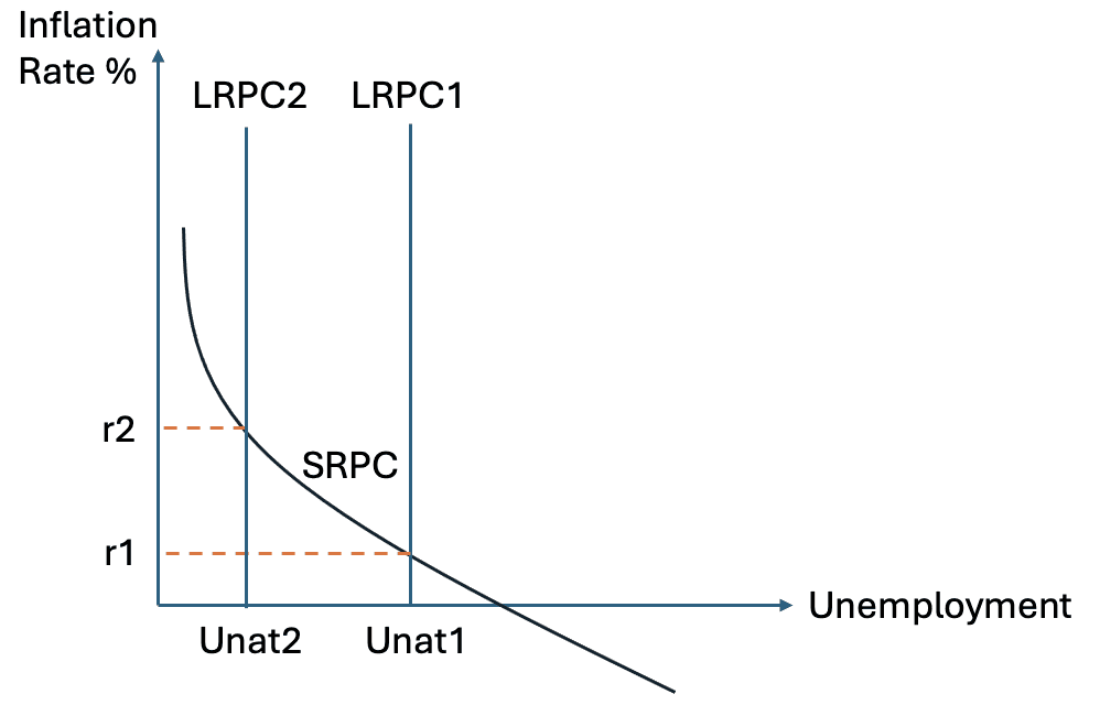
In the diagram, the long run Phillips curve shifts left, indicating a lower natural rate of unemployment. This shift allows the economy to achieve lower unemployment without generating accelerating inflation. In this way, supply side policies offer a way to reduce unemployment while maintaining price stability.

This highlights an important policy distinction. Demand side policies influence the position of the economy relative to the Phillips curve, while supply side policies influence the position of the curve itself. Sustainable improvements in employment therefore depend on addressing the underlying structural factors that determine the natural rate of unemployment.

Overall evaluation of the Phillips curve framework

The Phillips curve remains a valuable tool for understanding macroeconomic policy conflicts, even though the original idea of a stable trade off between unemployment and inflation has been rejected. Its modern interpretation emphasizes the role of expectations, the distinction between short run and long run outcomes, and the limits of policy intervention.

The framework explains why attempts to permanently trade higher inflation for lower unemployment are unsuccessful and why controlling inflation requires credibility and restraint. It also clarifies the role of supply side policy in achieving long term improvements in employment and output.

By highlighting the constraints policymakers face, the Phillips curve provides insight into the difficult choices involved in macroeconomic management. It shows that conflicts between objectives are unavoidable and that effective policy requires an understanding of both short run dynamics and long run structural conditions.