Introduction

The previous chapter examined how aggregate demand and aggregate supply interact to determine equilibrium real output and the overall price level. That framework explains how changes in spending or production conditions affect the economy at a point in time. However, it does not fully explain why relatively small changes in spending can sometimes lead to much larger changes in national income and output.

This chapter develops two related ideas that help explain these amplified effects. The first is the multiplier, which describes how an initial change in spending can lead to a larger final change in national income. The second is the accelerator, which explains how changes in output can influence investment and reinforce fluctuations in economic activity.

Both concepts build directly on the circular flow of income and the components of aggregate demand. They show how spending decisions are linked across households and firms, and how income generated in one part of the economy can lead to further rounds of spending elsewhere.

The Multiplier

The multiplier refers to the process by which an initial change in autonomous expenditure leads to a larger change in equilibrium national income. Autonomous expenditure is spending that does not depend on current income, such as government expenditure, investment, or exports.

The key idea behind the multiplier is that one person’s spending becomes another person’s income. When an initial injection of spending enters the circular flow of income, it generates income for households and firms. Those recipients then spend part of that income, generating further income for others. This process continues through multiple rounds, although each successive round becomes smaller.

The multiplier effect arises because households do not withdraw all of their additional income from the circular flow. Instead, they spend part of it on goods and services. As long as some of each increase in income is spent, total income will rise by more than the original injection.

How the Multiplier Works

To understand the multiplier, consider an increase in government expenditure. Suppose the government increases spending on infrastructure. Firms hired to carry out the work receive additional revenue. These firms then pay wages to workers and profits to owners. This income is now in the hands of households.

Households do not spend all of this additional income. They divide it between consumption and withdrawals. Withdrawals take the form of saving, taxation, and spending on imports. Consumption, however, represents spending on domestically produced goods and services and therefore generates further income.

The households who receive this second round of income again spend part of it and withdraw the rest. Each round of spending is smaller than the previous one because withdrawals reduce the amount that remains in the circular flow. Nevertheless, the cumulative effect of all rounds of spending is greater than the original increase in expenditure.

The multiplier therefore explains why an injection into the circular flow can have a magnified impact on equilibrium income and output.

Leakages and the Size of the Multiplier

The size of the multiplier depends on how much of each additional unit of income is withdrawn from the circular flow. These withdrawals are known as leakages. The main leakages are saving, taxation, and imports.

If households save a large proportion of any additional income, less income is passed on through consumption, and the multiplier effect is smaller. If households spend a large proportion of additional income on imported goods and services, income leaks out of the domestic economy, reducing the multiplier. Similarly, if a large proportion of additional income is taken in taxes, households have less disposable income available for consumption, reducing the multiplier effect.

The multiplier is therefore larger when leakages are small and smaller when leakages are large. This explains why the same increase in government spending can have different effects in different economies or at different times.

The Marginal Propensities

To analyse the multiplier more precisely, economists use marginal propensities. A marginal propensity measures how households respond to an increase in income.

The marginal propensity to consume is the proportion of an increase in disposable income that households spend on consumption. If households spend a high proportion of additional income, the marginal propensity to consume is high, and the multiplier effect is stronger.

The marginal propensity to save is the proportion of additional income that households save. The marginal propensity to import is the proportion of additional income spent on imported goods and services. The marginal propensity to tax is the proportion of additional income that is paid in taxes.

These marginal propensities determine the size of total withdrawals from the circular flow. The marginal propensity to withdraw is defined as the sum of the marginal propensities to save, tax, and import.

Because income must either be consumed or withdrawn, the marginal propensity to consume plus the marginal propensity to withdraw equals one.

Calculating the Multiplier

The multiplier can be calculated using the marginal propensity to withdraw. The numerical value of the multiplier is equal to one divided by the marginal propensity to withdraw.

This means that when withdrawals are large, the marginal propensity to withdraw is high and the multiplier is small. When withdrawals are small, the marginal propensity to withdraw is low and the multiplier is large.

An increase in autonomous expenditure therefore leads to a change in equilibrium income that is equal to the initial injection multiplied by the multiplier. This final change reflects the total impact of all rounds of spending in the circular flow.

The Multiplier and Aggregate Demand

The multiplier affects the position of the aggregate demand curve. When an injection such as government expenditure increases, aggregate demand shifts to the right. The multiplier means that the final shift in aggregate demand is larger than the initial increase in autonomous spending alone.

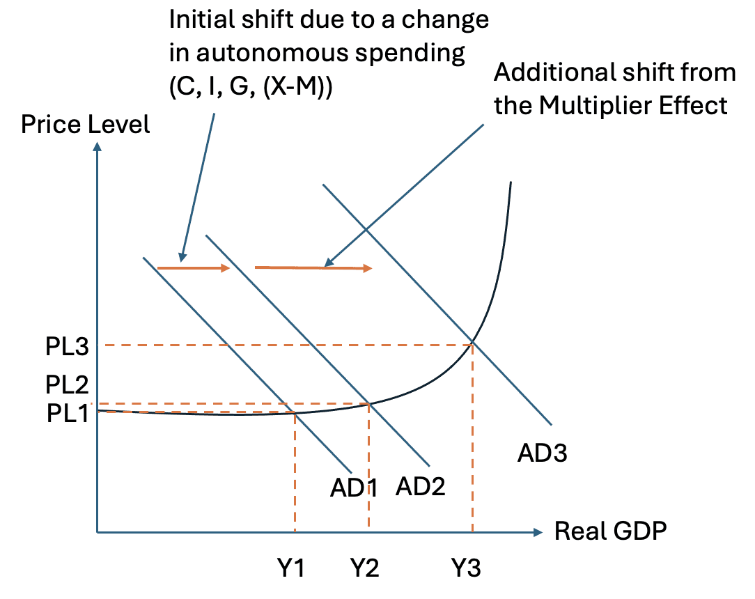
The initial increase in spending causes an initial rightward shift of aggregate demand. Subsequent rounds of induced consumption push aggregate demand further to the right. The full effect on equilibrium output and the price level depends on the shape of the aggregate supply curve and whether the economy is operating below or at full employment.

The Average and Marginal Propensities to Consume and Withdraw

To understand the size of the multiplier effect, it is necessary to examine how households allocate their income. Keynes’s analysis of consumption focused on the relationship between income and spending, and this relationship is captured through the concepts of average and marginal propensities.

The average propensity to consume refers to the proportion of total income that households devote to consumption. It is calculated by dividing total consumer expenditure by total income. This measure shows how much of income, on average, is spent rather than saved or withdrawn in other ways. As income rises, the average propensity to consume may change, reflecting shifts in household behaviour.

The marginal propensity to consume is more important for analysing the multiplier. It refers to the proportion of an increase in disposable income that households spend on consumption. If disposable income rises and households spend a large fraction of that additional income, the marginal propensity to consume is high. If they spend only a small fraction, the marginal propensity to consume is low.

Because the multiplier depends on how households respond to changes in income, it is the marginal rather than the average propensity that determines the strength of the multiplier effect.

Households do not devote all additional income to consumption. Some of it is withdrawn from the circular flow. These withdrawals take three main forms: saving, taxation, and spending on imports. Each of these has a corresponding marginal propensity.

The marginal propensity to save is the proportion of an increase in income that is saved rather than spent. Saving represents a withdrawal from the circular flow because it does not directly generate demand for goods and services.

The marginal propensity to tax is the proportion of an increase in income that is paid in taxes. Taxes reduce households’ disposable income and therefore reduce the amount available for consumption.

The marginal propensity to import is the proportion of additional income that is spent on imported goods and services. Spending on imports represents a leakage from the domestic circular flow because it generates income for producers abroad rather than domestically.

Together, these three marginal propensities determine the total marginal propensity to withdraw. The marginal propensity to withdraw is defined as the sum of the marginal propensities to save, tax, and import. It measures the proportion of additional income that does not lead to further rounds of domestic spending.

Because any increase in income must be either consumed or withdrawn, the marginal propensity to consume plus the marginal propensity to withdraw equals one. This identity reflects the fact that income is fully allocated between spending and leakages.

The Multiplier and Withdrawals

The size of the multiplier is inversely related to the marginal propensity to withdraw. When withdrawals are large, less income remains in the circular flow at each stage of the multiplier process. As a result, the chain of spending dies out more quickly, and the final increase in income is relatively small.

When withdrawals are small, a larger proportion of each increase in income is spent on domestically produced goods and services. This allows income to circulate for more rounds, increasing the overall impact of the initial injection.

This relationship explains why economies with high tax rates, high saving rates, or a strong tendency to import tend to have smaller multipliers. Conversely, economies where households spend a large proportion of additional income domestically tend to experience stronger multiplier effects.

The Multiplier and Macroeconomic Equilibrium

The multiplier affects how far aggregate demand shifts following a change in autonomous expenditure. An increase in government spending, investment, or exports initially shifts aggregate demand to the right. The multiplier process then amplifies this shift through induced consumption.

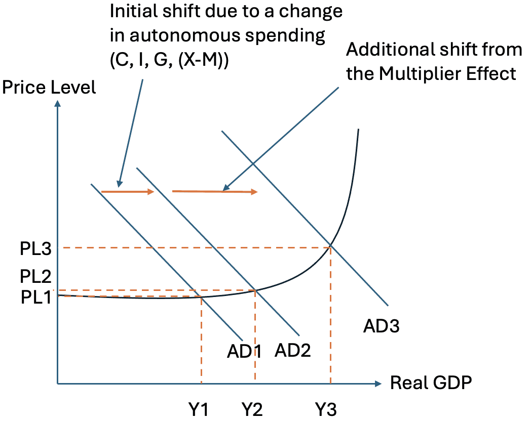
In the diagram, the initial increase in autonomous expenditure causes aggregate demand to move from its original position to a new position. As households receive additional income and spend part of it, aggregate demand shifts further to the right. The final position of aggregate demand reflects the full multiplier effect.

The multiplier influences the extent of the change in equilibrium output and income, but it does not guarantee a permanent change in macroeconomic equilibrium. As the economy adjusts, especially in the long run, other forces may offset the initial impact of the multiplier.

In particular, when the economy is at or near full employment, increases in aggregate demand are more likely to raise the price level than real output. In this case, the multiplier still operates, but its effect is reflected mainly in inflation rather than sustained increases in output.

The Accelerator

While the multiplier explains how an initial change in spending leads to a larger change in national income, the accelerator explains how changes in output can influence the level of investment undertaken by firms. The accelerator is based on the idea that firms’ investment decisions depend not on the absolute level of demand, but on changes in demand and output.

The accelerator refers to a theory in which the level of investment depends upon the change in real output. Firms invest in new capital when they expect demand for their products to rise and reduce investment when they expect demand to fall. This makes investment a volatile component of aggregate demand and helps explain why economic fluctuations can be amplified over time.

Some investment takes place simply to replace worn out or obsolete capital. However, the accelerator focuses on net investment that occurs when firms wish to expand productive capacity. This type of investment is driven by expectations about future demand.

How the Accelerator Works

To understand the accelerator, consider an economy that is recovering from a period of low demand and below full employment. As aggregate demand increases, real output begins to rise. Firms observe that demand for their products is increasing and may expect this increase to continue.

In response to this expected increase in future demand, firms may decide to expand their productive capacity. This requires investment in new capital, such as machinery, equipment, or buildings. As a result, investment spending increases.

The crucial point is that it is the change in output, rather than the level of output, that triggers this response. Even if output is still below its full employment level, a rise in output can generate a large increase in investment if firms expect demand to continue growing.

As output continues to rise, investment remains high. However, as the economy approaches full employment, the rate of growth of output may begin to slow. When firms observe that output growth is slowing, they may revise their expectations about future demand. As a result, investment spending may fall, even if output is still increasing.

This explains why investment can decline before the economy reaches a downturn and why investment is often the most volatile component of aggregate demand.

The Accelerator and Reversals in Economic Activity

The accelerator also operates in reverse. If firms observe a fall in demand or a slowdown in output growth, they may cut back investment sharply. Even a small fall in output can lead to a large reduction in investment spending if firms expect demand to continue falling.

This reduction in investment reduces aggregate demand, which may lead to a further fall in output. This creates a feedback process in which falling output leads to falling investment, which then reinforces the downturn in economic activity.

The accelerator therefore helps explain why economic expansions and contractions can be self reinforcing, at least for a period of time.

The Interaction Between the Multiplier and the Accelerator

The multiplier and the accelerator interact closely with each other. An initial increase in aggregate demand leads to an increase in output through the multiplier effect. As output rises, the accelerator induces an increase in investment. This increase in investment represents a further injection into the circular flow of income.

The additional investment then generates its own multiplier effect, leading to further increases in income and output. In this way, the multiplier and accelerator reinforce each other and can produce large fluctuations in economic activity.

However, the same process operates in reverse during a downturn. A fall in aggregate demand reduces output through the multiplier. Falling output reduces investment through the accelerator. The reduction in investment then triggers further multiplier effects, deepening the downturn.

This interaction helps explain cyclical fluctuations in output and income over time.

The Accelerator and Aggregate Supply

The accelerator has implications not only for aggregate demand but also for aggregate supply in the long run. When firms increase investment in response to rising output, they expand the productive capacity of the economy.

An increase in investment raises the capital stock. This increases the economy’s ability to produce goods and services and leads to an increase in the full employment level of real output. In terms of the aggregate supply framework, this is represented by a rightward shift of the long-run aggregate supply curve.

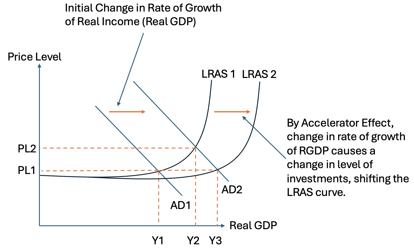
In the short run, increased investment raises aggregate demand and may lead to higher output and prices. In the long run, the expansion of productive capacity allows the economy to sustain a higher level of real output without generating inflationary pressure.

However, if firms come to expect that demand will no longer increase, they may reduce investment. In this case, the accelerator process goes into reverse, and the expansion of productive capacity slows or stops.

The Accelerator and Macroeconomic Equilibrium

The interaction of the accelerator with aggregate demand and aggregate supply affects the path of macroeconomic equilibrium. When rising demand triggers both multiplier and accelerator effects, equilibrium output may move closer to or beyond the full employment level in the short run.

Over time, as investment expands productive capacity, long-run aggregate supply increases. This allows the economy to settle at a higher level of real output in the long run.

If expectations change or demand growth slows, the accelerator effect weakens. Investment falls, and the economy may experience a slowdown or contraction before long-run equilibrium is restored.

An Output Gap

The concept of an output gap is used to describe the difference between the actual level of real output produced by the economy and the level of output that would be produced if the economy were operating at full employment. The output gap therefore measures how far the economy is operating away from its productive capacity.

The full employment level of output is the level of real GDP that occurs when all factors of production are fully employed. This does not imply zero unemployment, but rather that the economy is operating without cyclical unemployment and that labour and capital are being used as intensively as is sustainable.

The output gap can be either positive or negative. A positive output gap occurs when actual real GDP is above the full employment level. In this situation, the economy is operating beyond its sustainable capacity. Firms may be using overtime, running machinery for longer hours, or relying on short term measures to meet high demand. A negative output gap occurs when actual real GDP is below the full employment level. In this case, there is spare capacity in the economy, with unemployed labour and underutilised capital.

Identifying an Output Gap Using the AD and AS Model

The output gap can be identified using the aggregate demand and aggregate supply framework by comparing the equilibrium level of output with the full employment level of output.

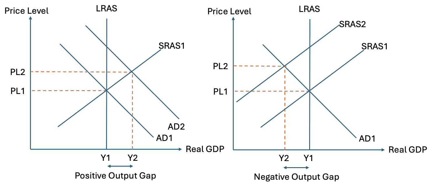
In the diagram, the vertical axis shows the price level and the horizontal axis shows real GDP. The long-run aggregate supply curve represents the full employment level of output. If aggregate demand intersects aggregate supply at a point to the right of long-run aggregate supply, the equilibrium level of output is above full employment and there is a positive output gap. If the intersection occurs to the left of long-run aggregate supply, the equilibrium level of output is below full employment and there is a negative output gap.

A positive output gap may arise following an increase in aggregate demand when the economy is already close to full employment. In the short run, firms are willing to increase output in response to higher demand. However, this situation is unsustainable in the long run. Rising costs and wages eventually reduce short-run aggregate supply, bringing output back toward the full employment level.

A negative output gap may arise following a fall in aggregate demand. This could result from a decline in consumption, investment, government expenditure, or exports. In the short run, firms reduce output and employment. Whether the economy returns quickly to full employment depends on how wages, prices, and expectations adjust over time.

Identifying an Output Gap Using the Production Possibility Curve

The output gap can also be illustrated using the production possibility curve. The production possibility curve shows the maximum combinations of two types of goods that an economy can produce when all resources are fully employed and used efficiently.

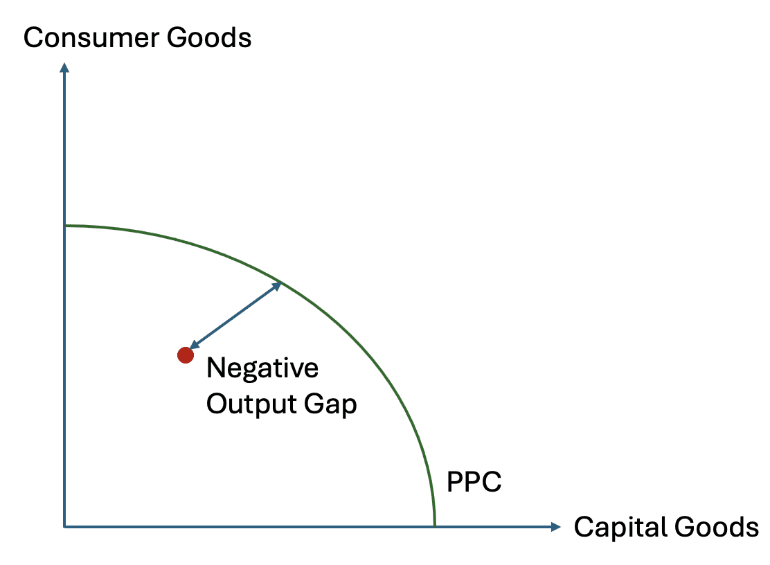
Any point on the production possibility curve represents full employment of resources. If the economy is producing at a point inside the curve, it is operating below its potential capacity. This corresponds to a negative output gap. Resources are unemployed or underutilised, and it is possible to increase output without sacrificing production of other goods.

If the economy is producing at a point on the curve, there is no output gap. The economy is operating at full employment. Points outside the curve are unattainable given current resources and current technology.

The production possibility curve therefore provides an alternative way of visualising the output gap, consistent with the aggregate demand and aggregate supply framework.

Causes of an Output Gap

An output gap can arise from changes in aggregate demand. A positive output gap may occur when aggregate demand increases while the economy is already at full employment. For example, an increase in government expenditure or exports can push real GDP above the full employment level in the short run.

A negative output gap may occur when aggregate demand falls. This could be due to pessimistic expectations among firms leading to lower investment, a fall in exports, or a reduction in government spending. External shocks that reduce demand can also generate a negative output gap.

The persistence of an output gap depends on how the economy adjusts over time. Under neoclassical assumptions, wages and prices adjust to restore full employment relatively quickly. Under Keynesian assumptions, downward adjustments in wages and prices may be slow, allowing a negative output gap to persist.

Consequences of an Output Gap

A positive output gap places upward pressure on prices. As firms operate beyond normal capacity, costs rise and inflationary pressure builds. Over time, these cost increases reduce short-run aggregate supply and bring output back toward the full employment level.

A negative output gap is associated with unemployment and lost output. Firms operate below capacity, and resources are wasted. If the negative output gap persists, there may be long lasting effects on skills, investment, and productive capacity.

The impact of an output gap therefore depends on its size, its duration, and the way the economy responds to changes in demand and supply.

Evaluation of the Output Gap

The significance of an output gap depends on how the economy adjusts over time and on the assumptions made about the flexibility of wages and prices. Different economic perspectives lead to different conclusions about whether an output gap is temporary or persistent, and about the role of policy in addressing it.

Under neoclassical assumptions, the economy is viewed as tending naturally toward its full employment level of output. If an output gap emerges, it is assumed to be short lived. A negative output gap creates downward pressure on wages and other input costs as firms face weak demand and excess capacity. As costs fall, firms regain profitability and increase output. This process shifts short run aggregate supply to the right until output returns to the full employment level.

In this view, the economy adjusts relatively quickly, and output gaps are mainly a short run phenomenon. Because market forces are assumed to restore equilibrium, there is limited justification for sustained policy intervention. Attempts to stimulate demand may only affect the price level once full employment is restored.

Under Keynesian assumptions, the adjustment process may be much slower. Wages may be downwardly inflexible due to contracts, minimum wages, or institutional factors. Firms may also be reluctant to cut prices in the face of weak demand. As a result, a negative output gap can persist for an extended period.

In this case, the economy may settle at an equilibrium level of output below full employment. Aggregate demand intersects aggregate supply in the upward sloping section of the long run aggregate supply curve. The output gap remains negative, and unemployment persists. Without an increase in aggregate demand, the economy may not return to full employment on its own.

This difference in assumptions leads to contrasting views on the role of demand management. Under Keynesian assumptions, an increase in aggregate demand may be required to close a negative output gap. Such an increase could arise from higher government expenditure, increased investment, or stronger exports. Through the multiplier, this increase in demand can raise output and reduce unemployment.

The evaluation of a positive output gap follows a similar logic. Under neoclassical assumptions, operating above full employment is unsustainable and quickly leads to rising wages and costs. These cost pressures shift short run aggregate supply to the left, reducing output back to its full employment level. The main long run effect is higher prices rather than permanently higher output.

Under Keynesian assumptions, a positive output gap may persist for a period, but it is still expected to generate inflationary pressure over time. As resources become increasingly scarce, costs rise and firms reduce output. Eventually, output moves back toward the full employment level, though the adjustment path may be uneven.

The importance of the output gap also depends on whether changes in aggregate demand are temporary or permanent. A temporary increase in demand may generate only a short run output gap, with little long term effect on real output. A permanent change in demand may interact with the multiplier and accelerator to influence investment and productive capacity, affecting long run aggregate supply.

Overall, the concept of the output gap provides a useful way of linking short run fluctuations in output to longer run economic performance. It highlights the role of aggregate demand in driving deviations from full employment and the conditions under which these deviations may persist.