The Demand for Labor as a Derived Demand

The demand for labor arises because labor is one of the key factors of production used in the creation of goods and services. Firms require labor not for its own sake, but for the productive power it brings. A firm hires workers to help produce output that can later be sold, and the revenue from this output is the true reason labor is demanded. Economists describe this as derived demand, because the demand for a factor of production depends not on the direct utility or satisfaction it provides, but on the demand for the final goods and services that the factor helps to produce. Labor is valuable to a firm only because consumers wish to buy the products or services that labor contributes to creating.

When a firm undertakes production, it must organize the various factors of production: land, labor, capital, and enterprise. Each factor receives its corresponding reward: rent for land, wages for labor, interest or dividends for capital, and profit for enterprise. Labor, therefore, represents one essential input in this wider process of production. But unlike land or capital, laborers ' human effort — physical and mental — is applied to the production process. This makes labor distinctive among the factors because it is not only a cost to the firm but also a determinant of how much output the firm can generate.

In considering why labor demand is derived, it is helpful to think of the link between product markets and factor markets. Firms produce goods and services to meet the demand of consumers in the product market, and to do so, they must hire labor in the factor market. If demand for the firm's output rises, the firm will seek to expand production. To increase production, it will hire more workers, increasing its demand for labor. Conversely, if demand for its output falls, the firm will need fewer workers. This chain of reasoning shows that the demand for labor is indirectly determined by the demand for the firm's final product.

To illustrate, consider a firm that manufactures cricket bats. The firm does not hire labor because it has any intrinsic need for employees, but because it needs workers to operate its machinery and produce the bats that consumers will buy. The firm earns profit by selling the bats, and the number of workers it hires depends on the quantity of bats it expects to sell. If demand for cricket bats increases — perhaps because of a surge in interest in the sport — the firm will employ more workers to increase output. If sales fall, employment will be reduced. This example demonstrates that the demand for labor exists only because of the demand for what labor helps to make.

This notion of derived demand is a fundamental principle in labor economics. It underpins the entire analysis of how firms decide how many workers to hire, what wages they are willing to pay, and how employment levels in an economy fluctuate. The labor market cannot be analyzed in isolation from the product markets it serves. A firm's willingness to employ additional workers depends on the revenue that each worker is expected to generate. This connects directly to the concept of the marginal revenue product of labor, which will be explored later in this chapter, but the key foundation is that labor is only valuable to the extent that it contributes to output and revenue.

An important implication of derived demand is that changes in consumer demand, technology, or production methods will all influence employment. When consumer preferences shift, firms must adjust their production accordingly, and this adjustment alters the demand for workers in affected industries. For example, if consumers demand more digital products and fewer printed goods, firms in the printing industry will reduce employment while firms in the technology sector expand it. The underlying cause, however, is always traced back to the demand for the final goods.

Understanding this link between output markets and the demand for labor also clarifies why wages and employment can vary so much across occupations. Occupations in which the product has high and sustained demand — such as technology or professional sports — will generate higher derived demand for labor, leading to higher wages. Occupations where demand for the final product is limited or falls quickly, such as certain manufacturing or routine services, will experience weaker labor demand and lower wages. These variations are not primarily about the inherent worth of the workers but about the economic value of what they help produce.

While derived demand connects labor markets to product markets, it is also essential to recognize that the labor market itself is not uniform. In reality, there is no single labor market for an entire economy. Instead, there are numerous sub-markets divided by occupation, skill level, geography, and industry. A firm may face different conditions when hiring engineers compared with hiring accountants or manual workers, even if both are employed within the same company. These sub-markets exist because workers differ in their skills and mobility, and because demand for their services depends on the specific output they help to create.

Geographical differences can also create distinct labor markets. For instance, firms may find it easier to hire certain types of workers in one region than in another. Some workers may also be less mobile, meaning they are unable or unwilling to move to locations where their skills are more in demand. In this case, the derived demand for labor interacts with mobility constraints, producing regional variations in employment and wages. A firm may therefore operate in several sub-markets simultaneously, each with its own equilibrium wage rate and level of employment, depending on local and occupational factors.

Derived demand also helps to explain why changes in technology or capital investment can alter employment levels. When firms adopt new machinery or production techniques, they may substitute capital for labor if the new technology makes production more efficient. In such cases, even if consumer demand for the product remains unchanged, the firm's derived demand for labor falls because it can now produce the same output with fewer workers. Alternatively, if technological progress raises productivity, making workers more efficient, firms may be able to expand output and thus hire more labor overall.

It is also important to distinguish between labor demand in the short run and the long run. In the short run, a firm may treat some factors of production as fixed — typically capital — and vary only the amount of labor it employs. When product demand increases, the firm responds by hiring more workers, assuming existing capital can accommodate the additional labor. Over the longer run, however, firms can alter both capital and labor inputs, and this flexibility allows them to adjust production more efficiently. The derived demand for labor is therefore influenced by both time horizons and production flexibility.

Because the demand for labor depends on output demand, the labor market is closely linked to overall economic conditions. During periods of economic growth, when consumer spending and investment rise, firms experience greater demand for their products and therefore expand employment. During recessions, when output falls, labor demand contracts as firms cut back production. These cyclical fluctuations are transmitted from product markets to labor markets through the mechanism of derived demand.

Derived demand thus connects individual employment decisions to the wider performance of the economy. A firm will not hire labor simply to provide work or maintain employment. It hires labor only if doing so contributes to the profitability of the firm. The amount of labor demanded depends on the value of what each additional worker produces, measured in terms of revenue from the final good or service. For this reason, the analysis of labor demand must always begin with the principle that the demand for labor is derived — it is determined by the demand for the output that labor helps to produce.

The Demand Curve for Labor and the Marginal Revenue Product

The relationship between the firm's demand for labor and the productivity of that labor is central to understanding how wages and employment are determined. Labor, like all factors of production, contributes to output, but the firm values labor not for the physical goods or services it produces directly, but rather for the revenue those outputs generate when sold. The firm's willingness to hire additional workers depends on how much extra revenue it gains from each new unit of labor employed. This relationship forms the foundation of the marginal revenue product of labor, abbreviated as MRP.

The concept of marginal revenue product combines two ideas that are essential for analyzing factor demand: the marginal physical product of labor (MPP) and the marginal revenue (MR). The marginal physical product of labor refers to the extra quantity of output produced when one more unit of labor is employed, keeping all other inputs, such as capital, constant. This concept was introduced earlier through the law of diminishing returns, which explains that as more units of a variable factor, such as labor, are added to a fixed factor, such as capital, the additional output gained from each successive worker will eventually begin to fall. This decline in additional output reflects the limits of productive capacity when some inputs are fixed.

While the marginal physical product measures physical output, what matters to a profit-seeking firm is not merely the quantity produced but the revenue that quantity earns when sold. Hence, the marginal revenue product measures the extra revenue generated by employing an additional unit of labor. It is found by multiplying the marginal physical product by the marginal revenue received from selling the output. In a perfectly competitive product market, marginal revenue is constant and equal to price, so the MRP simply equals the MPP multiplied by price. In an imperfectly competitive market, however, marginal revenue falls as output increases because the firm must lower its selling price to sell more units, so the MRP curve will fall more steeply than the MPP curve.

The demand curve for labor is derived from the MRP schedule. Each point on the MRP curve represents the additional revenue the firm earns from employing one more unit of labor. The firm will only hire workers up to the point where the value of their marginal revenue product equals the cost of employing them, which is the wage rate. The MRP curve, therefore, shows the maximum wage that the firm is willing to pay for any given quantity of labor. Because the marginal revenue product diminishes as more labor is employed — due both to the law of diminishing returns and, in imperfect competition, to the falling marginal revenue of the product — the MRP curve slopes downwards from left to right.

The diagram of the demand curve for labor shows the marginal revenue product curve on a graph with the quantity of labor on the horizontal axis and wage or marginal revenue product on the vertical axis. The curve slopes downward, illustrating that as more labor is hired, the additional revenue generated by each worker declines. This decline occurs because the productivity of successive workers falls once the firm has already employed the most efficient combination of labor and capital, and also because additional output must often be sold at lower prices. The downward slope, therefore, captures both technological limits and market conditions.

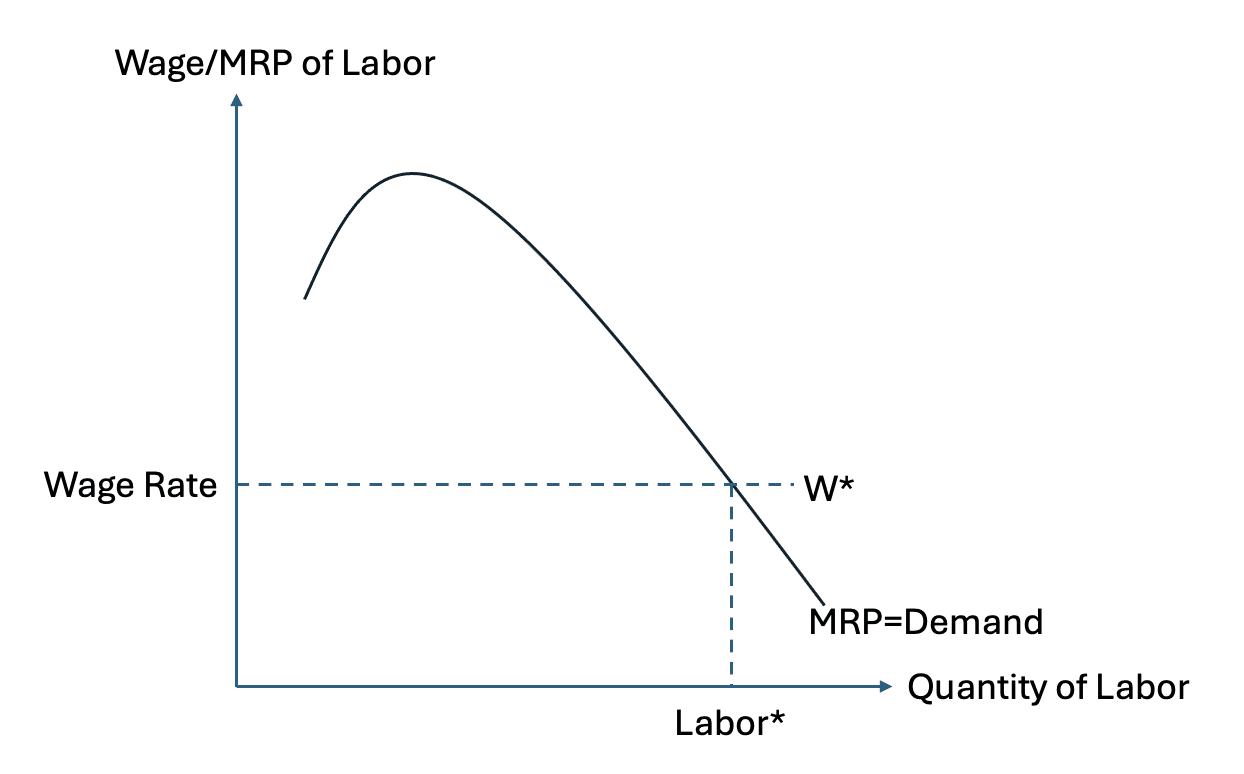
When the firm faces a given market wage rate, it will employ labor up to the point where the MRP equals that wage. Suppose the going wage rate in the market is W*. The firm will employ labor* units at the intersection between the wage line and the MRP curve. If the wage were to rise, fewer workers would be hired because the cost of labor would exceed its marginal revenue product for some workers. Conversely, if the wage were to fall, employment would expand since it would now be profitable to employ additional workers. The MRP curve, therefore, also represents the firm's demand curve for labor, showing the quantity of labor demanded at different wage levels.

This reasoning assumes that the firm is a price taker in the labor market — that is, it must accept the prevailing market wage and cannot influence it. In such a situation, the firm's choice is limited to deciding how much labor to hire at that wage, not what wage to pay. Because the wage represents the marginal cost of labor to the firm, the point where the MRP equals the wage identifies the profit-maximizing level of employment.

The link between the MPP, MR, and MRP can be understood step by step. As a firm increases its labor input, the total output produced initially rises rapidly. During this stage, both the marginal physical product and the marginal revenue product of labor increase because each additional worker adds more output than the previous one. Eventually, however, as the firm employs more workers with a fixed amount of capital, congestion and inefficiency set in. Each additional worker contributes less additional output, and so the marginal physical product begins to decline. Because the marginal revenue product is derived from the marginal physical product, it also declines.

The decline in MRP gives the demand curve for labor its downward slope. It reflects the diminishing benefit to the firm from employing successive units of labor. Even though each worker is paid the same market wage, the extra revenue the firm gains from each additional worker is less than that from the previous one. Rational firms therefore employ workers only up to the point where hiring another worker would no longer add to profits — where the marginal revenue product just equals the wage rate.

In a diagram of the marginal revenue product of labor, the vertical axis represents the value of the marginal revenue product, and the horizontal axis represents the quantity of labor employed. The downward-sloping MRP curve cuts the horizontal line representing the market wage rate at the equilibrium quantity of labor demanded. To the left of this intersection, MRP is higher than the wage, meaning it is profitable to hire more labor. To the right, MRP is lower than the wage, meaning additional hiring would reduce profit. Hence, equilibrium employment occurs exactly where the two are equal.

It is also possible to see the MRP concept numerically. Suppose the firm sells its output for a fixed price. As it increases the number of workers, total output rises, but the additional output produced by each worker decreases due to diminishing returns. Multiplying each worker's marginal product by the constant price gives the marginal revenue product for that worker. The firm compares this figure with the wage. If MRP exceeds the wage, the firm earns profit from employing that worker. If MRP is below the wage, employing that worker reduces profit. This numerical relationship determines the optimal number of workers.

Although this analysis is framed in terms of a single firm, it extends to the whole industry. The industry's demand curve for labor is obtained by summing the MRP curves of all firms horizontally — that is, by adding the quantities of labor each firm demands at every possible wage. The industry demand for labor, therefore, slopes downward as well, reflecting the same diminishing marginal productivity principle operating across firms.

It is crucial to note that the MRP concept does not suggest that workers are paid according to their moral worth or effort. It simply expresses how the value of labor is determined in a market economy. A worker who contributes to producing goods that sell for high prices will tend to have a high marginal revenue product, while a worker whose output is sold at lower prices will have a lower MRP. The MRP theory, therefore, provides an objective, revenue-based explanation of how firms decide on employment levels and wage payments.

This framework also helps explain why demand for labor differs between industries and between skill groups. Jobs that contribute to the production of highly valued output — such as specialized manufacturing or advanced technology — will have higher MRP values, leading firms to offer higher wages to attract workers. Jobs that add less value to output, or where the market price of the product is low, will generate lower MRP and therefore support lower wages. In every case, the key principle is that the firm hires labor up to the point where the marginal revenue from the last worker employed equals the wage paid to that worker.

The downward-sloping nature of the MRP curve captures both the productivity side and the revenue side of labor demand. Productivity diminishes as more labor is applied to a fixed amount of capital, while the revenue gained from selling additional output often falls as well. The combined effect ensures that each additional worker contributes less to total revenue than the one before. This ensures that the firm's demand for labor is inversely related to the wage rate.

By combining the concepts of marginal physical product, marginal revenue, and marginal revenue product, economists can therefore explain how the demand curve for labor is formed, why it slopes downward, and how the firm decides the level of employment that maximizes profit under competitive conditions.

Employment and the Wage

The firm's decision about how much labor to employ depends on the relationship between the additional revenue gained from labor and the cost of employing it. The marginal revenue product of labor measures the extra revenue that one additional unit of labor brings, while the wage rate represents the cost of that labor to the firm. A profit-maximizing firm will hire labor up to the point where these two values are equal. At that point, the revenue gained from the last unit of labor exactly matches its cost, so there is no incentive to hire more or fewer workers.

This decision can be understood by considering the marginal cost of labor. In a competitive labor market, firms take the wage rate as given because each individual firm is too small to influence the market wage. It can hire as many workers as it wishes at that rate, but if it tries to offer a lower wage, it will not attract workers, and if it offers a higher wage, it would only be unnecessarily increasing costs. Therefore, for a firm operating under perfect competition in the labor market, the wage rate acts as a constant marginal cost of labor.

On a diagram, the quantity of labor is shown on the horizontal axis and the wage rate on the vertical axis. The horizontal line drawn at the level of the going wage W∗ represents the firm's marginal cost of labor (MCL​). The marginal revenue product curve, MRP(L), slopes downward, reflecting the diminishing additional revenue generated by employing successive units of labor. The intersection of the wage line W∗ and the MRP(L) curve gives the equilibrium level of employment L∗. This point identifies the firm's optimal employment decision under competitive conditions.

To see why this outcome is logical, consider what would happen if the firm hired fewer or more workers than Labor*. If the firm employed fewer workers, the marginal revenue product of the last worker would exceed the wage. That means the firm could gain additional profit by hiring more labor, since each new worker would add more to revenue than to cost. Hiring would continue until this profit opportunity disappeared. On the other hand, if the firm hired more workers than labor*, the marginal revenue product of the last worker would fall below the wage. In that case, each extra worker would cost more than the revenue they produced, so the firm would reduce employment until MRP once again equalled the wage. The equality of MRP and the wage, therefore, defines the profit-maximizing equilibrium.

This logic is illustrated in the diagram below, which depicts the firm’s labor demand under conditions of perfect competition. The horizontal line represents the wage rate W∗. The downward-sloping MRP curve shows how the value of the marginal product of labor diminishes as more labor is hired. The firm employs labor up to point labor*, where the two curves meet. Beyond this point, the additional cost of employing labor exceeds the extra revenue it generates.

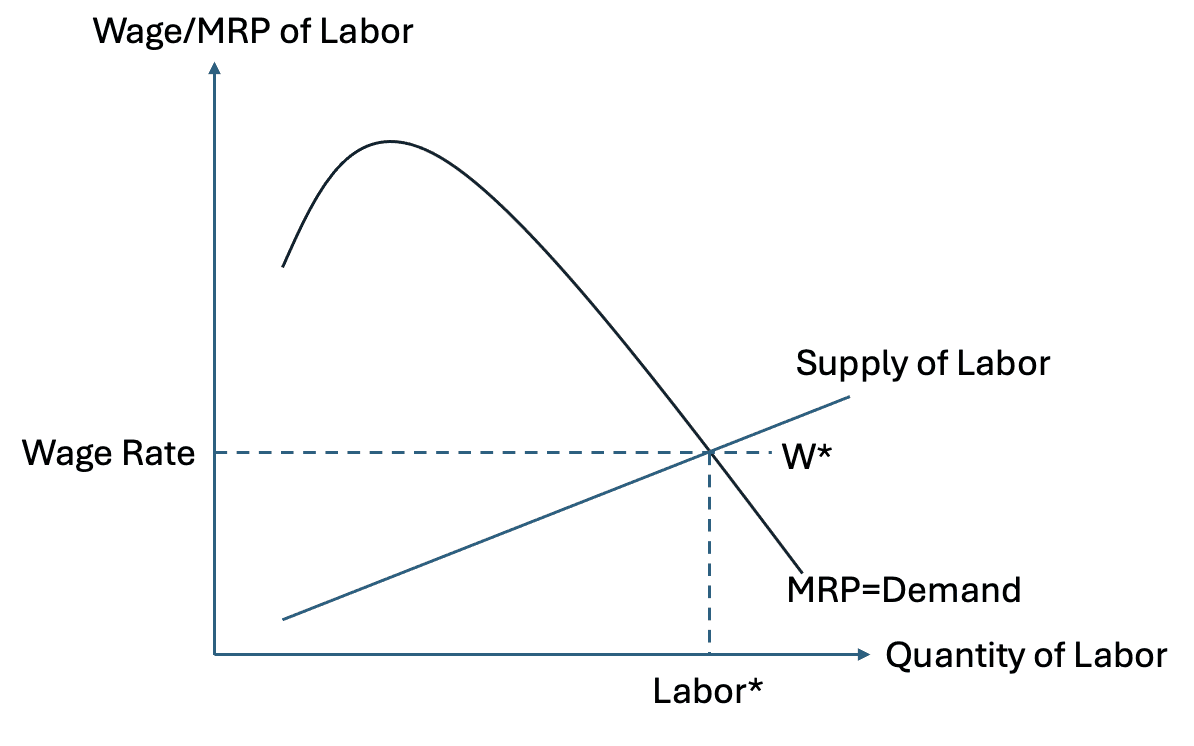
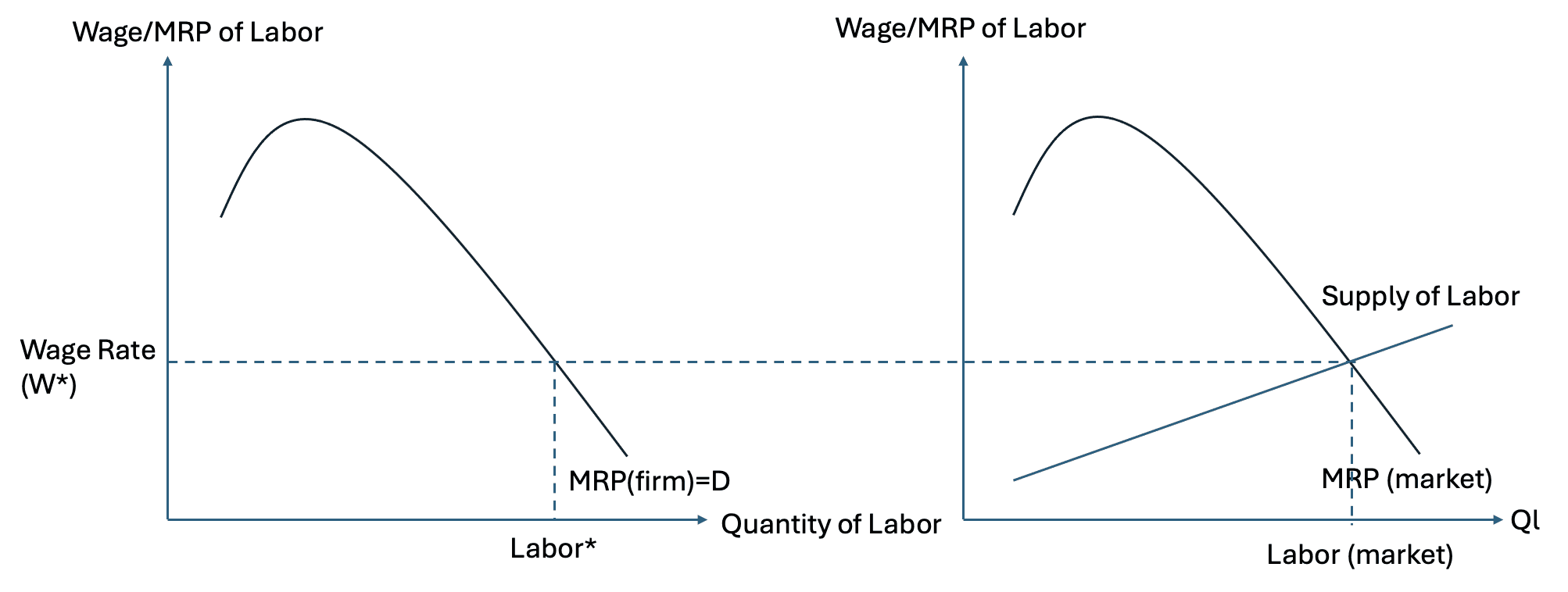
The wage rate itself, however, is determined by the interaction of demand and supply in the broader labor market, not by the decisions of any individual firm. Each firm is a wage taker. It is the outcome of the broader market for labor where many firms demand labor and many workers supply it. For the single firm, the wage is a parameter that cannot be altered. The only decision is how much labor to hire at that wage. This is why the horizontal line in the diagram represents the marginal cost of labor for the firm.

The total demand for labour in the market comes from the sum of all firms’ MRP curves, while the supply of labour reflects the willingness of workers to offer their time and skills at different wage levels. The intersection of these two market forces sets the equilibrium wage rate W∗. Individual firms then respond by hiring labour up to the point where their own MRP equals this market wage.

Within this framework, the firm’s wage payments represent its major variable cost. If the wage rate increases, the marginal cost of employing labour rises, and the equilibrium employment level falls. If the wage rate decreases, the marginal cost of labour falls, and the firm expands employment. The relationship between wages and employment is therefore inverse, holding productivity and output price constant.

The marginal cost of labour, as used in this analysis, should not be confused with total labour cost. The marginal cost refers specifically to the cost of employing one extra unit of labour, while total labour cost refers to the total wages paid for all employees. At the profit-maximising equilibrium, the marginal cost of labour equals the marginal revenue product, but total revenue and total cost can still differ substantially. The area between the wage line and the MRP curve up to the equilibrium quantity represents the firm’s total surplus from employing labour.

Therefore, the equilibrium condition (when the firm maximizes profit) can also be expressed:

• MRPL = MCL = W*

where MRPL​ is the additional revenue generated by the last unit of labor, MCL​ is the marginal cost of that labor, and W∗ is the market wage. This equality ensures that every unit of labor contributes exactly its cost to revenue, thereby maximizing total profit.

It is important to recognize that this analysis assumes perfect competition in both the product and labor markets. Under such conditions, the firm faces a perfectly elastic supply of labor at the given wage, and marginal revenue is constant because it is a price taker in the product market. In the real world, these assumptions may not always hold, but they provide a benchmark for understanding how firms decide on employment when they cannot influence either the wage rate or the price of output.

The same reasoning explains why changes in productivity or output demand will shift the demand for labour. If labour becomes more productive, the MRP curve shifts upward, meaning that at any given wage, labour now generates more revenue for the firm. This encourages the firm to hire more workers, increasing equilibrium employment. Conversely, if productivity falls, or if demand for the firm’s output decreases, the MRP curve shifts downward, reducing equilibrium employment even if the wage remains unchanged.

From the perspective of the firm, the MRP curve provides all the information needed to determine employment at a given wage. The downward slope indicates that labour becomes less valuable at the margin as more of it is used, and the point of intersection with the wage line determines the optimal workforce size. This analysis also explains how wages influence firms’ decisions across industries. High-wage sectors will employ fewer workers unless those workers have proportionately higher productivity, while lower-wage sectors can afford to employ more workers, provided their productivity justifies the wage.

The equality of MRP and the wage also links labor demand to overall efficiency. In competitive markets, each worker is paid a wage equal to their marginal contribution to revenue, ensuring that resources are allocated efficiently among firms. If a worker could earn more by moving to another firm, they would do so until MRP values were equalised across the market. This mobility of labor helps maintain efficiency, as workers shift to firms and industries where their contributions to output are most valuable.

This also shows how wages are price signals. A rising wage signals labor scarcity relative to demand, prompting firms to economize on labor or invest in labor-saving capital. A falling wage signals excess supply of labor, encouraging firms to expand employment. Thus, the wage rate functions as a coordinating mechanism between workers’ willingness to supply labor and firms’ demand for it.

It is helpful to connect this condition to the earlier definition of marginal revenue product. The marginal revenue product of labor equals the marginal physical product of labor multiplied by the marginal revenue from selling the extra output. If the firm sells its product in a competitive product market, marginal revenue equals the market price. In that case, the marginal revenue product of labor equals the marginal physical product multiplied by the price of the product. If the firm faces a downward sloping demand curve for its product, marginal revenue is lower than price and falls as output expands, so the marginal revenue product of labor declines more quickly as employment rises. In either case, the firm hires labor up to the point where the value of the extra output produced by the last unit of labor just covers the wage paid to that unit.

Let's illustrate this with an example: suppose a firm can sell each unit of its product at a fixed price of five pounds. As the firm increases labor from zero to one unit, output rises from zero to seven units. The marginal physical product of the first unit of labor is seven. The marginal revenue product is seven multiplied by five which equals thirty-five. When labor increases from one to two units, output rises from seven to fifteen units. The marginal physical product of the second unit is eight, and the marginal revenue product is eight multiplied by five, which equals forty. When labor increases from two to three units, output rises from fifteen to twenty-two. The marginal physical product of the third unit is seven and the marginal revenue product is thirty-five. As labor increases further, the marginal physical product declines to five, then to two, and the corresponding marginal revenue products decline in the same proportions. The firm compares each marginal revenue product with the wage. It hires labor up to the point where the last worker's marginal revenue product just equals the wage.

This shows diminishing marginal returns to labor when capital is held constant. The pattern is that the marginal physical product rises at first, reaches a peak, and then falls as congestion sets in. Because marginal revenue product is the product of marginal physical product and marginal revenue, it follows the same general shape. The employment rule based on equality with the wage , therefore, provides the exact point where the firm should stop increasing labor.

The equality between marginal revenue product and the wage also carries an efficiency meaning. When each worker is paid a wage equal to the value of the extra output that worker produces, labor is allocated to the uses where it contributes the most to revenue. If a worker could generate a higher marginal revenue product at another firm, that firm would be willing to match or exceed the current wage, and the worker would have an incentive to move. This movement continues until marginal revenue products are aligned with wages across firms operating under the same market wage. The result is an efficient distribution of labor across firms and sectors consistent with the conditions laid out in this chapter.

Finally, it is important to recognize the time horizon that underlies the diagram. In the short run, some inputs, such as capital, are fixed. The firm varies labor and observes diminishing marginal product as employment rises. In the longer run, firms can adjust both labor and capital, and this will shift the marginal revenue product schedule. The decision rule remains the same. For any given wage, the firm chooses the level of labor where the marginal revenue product equals that wage.

Factors affecting the position of the demand for labor curve

The demand curve for labor shows how many units of labor a firm is willing to employ at different wage levels, assuming all other factors remain constant. The curve slopes downward because of diminishing marginal returns and because each extra worker adds less additional revenue than the previous one, once some inputs, such as capital, are fixed. However, in reality other variables do not remain fixed. Several factors can cause the entire demand for labor curve to shift to a new position. A shift means that at every possible wage, the firm wishes to employ either more or fewer labor than before. These changes occur because the marginal revenue product of labor depends on both how productive workers are and how much revenue their output earns when sold. Any factor that changes either productivity or the value of output will shift the curve.

1. Changes in the productivity of labor

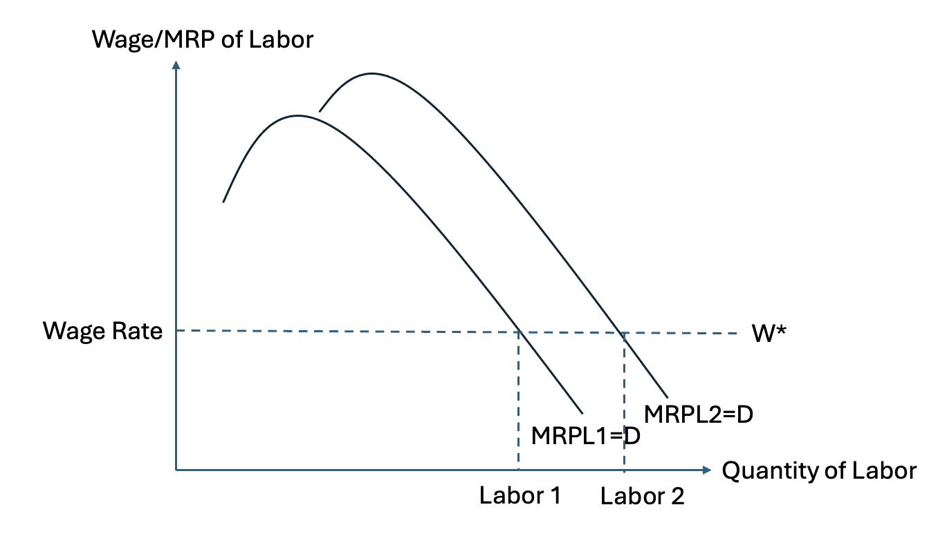
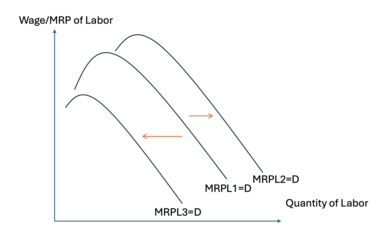
The productivity of labor measures how much output each worker can produce in a given period of time. If workers become more efficient, each unit of labor contributes more to total output. When productivity rises, the marginal physical product of labor increases at every level of employment. Since marginal revenue product equals marginal physical product multiplied by marginal revenue, the marginal revenue product of labor increases at all levels as well. The result is that the entire demand for labor curve shifts to the right. At any given wage, the firm now finds it profitable to hire more workers because each worker generates more revenue than before.

An increase in productivity can result from several sources, such as better training, improved production organization, or technological improvements that make labor more effective. For example, if new equipment allows workers to produce more goods in the same amount of time, the firm’s marginal physical product of labor rises. The revenue per worker, therefore, increases, causing the marginal revenue product and, hence, the demand for labor to increase. A fall in productivity has the opposite effect. If workers become less efficient, or if production is disrupted, each worker produces less output and the marginal revenue product at every level of employment falls. The demand for labor curve shifts to the left.

2. Changes in the demand for the firm’s product

Because the demand for labor is derived from the demand for output, any change in the demand for the firm’s product affects labor demand. If consumers demand more of the product, the firm increases production to meet this higher demand. To expand production, it must hire more labor. The increase in product demand also raises marginal revenue because each additional unit of output can be sold at the same or possibly a higher price. This increase in marginal revenue causes the marginal revenue product of labour to rise. At any given wage, the firm now finds it profitable to employ more labor, shifting the demand for labor curve to the right.

If demand for the firm’s product falls, the opposite occurs. The firm sells fewer units of output and may have to reduce its price to maintain sales. Marginal revenue falls, and consequently, the marginal revenue product of labor falls at every level of employment. The firm’s demand for labour curve shifts to the left. At each possible wage, fewer workers are now employed because their additional revenue to the firm has decreased.

In this way, the conditions in the product market directly determine employment outcomes. When demand for output strengthens, labor demand expands. When demand weakens, labour demand contracts. This link ensures that employment levels in each industry reflect consumer preferences for the goods and services those industries produce.

3. Changes in the price of other factors of production

Labour rarely operates in isolation. Firms combine labour with capital, land, and enterprise to produce output. A change in the price of any of these other factors can affect labor demand. The direction of the effect depends on whether the factors are substitutes or complements in production.

If labor and capital are substitutes, a rise in the cost of capital makes labor relatively cheaper. Firms substitute labor for capital by hiring more workers instead of purchasing new machinery. This increases the demand for labor, shifting the demand for labor curve to the right. Conversely, if the price of capital falls, firms find it cheaper to invest in machinery or automation rather than employ additional workers. The demand for labor shifts to the left.

If labor and capital are complements, the relationship is reversed. When the cost of capital rises, firms may reduce output because using both factors together becomes more expensive. In this case, the demand for labor falls along with the use of capital. When the cost of capital falls, firms can expand production by using more of both inputs, increasing the demand for labor.

These relationships illustrate that changes in the prices of other factors do not operate in one direction. The key determinant is whether labor and those factors work together or can replace one another in production.

4. Changes in technology

Technological progress can also shift the demand for labor curve. The effect depends on how the new technology interacts with labor. If the technology enhances labor efficiency, making workers more productive, the marginal physical product of labor rises, and hence the marginal revenue product rises at every level of employment. This shifts the demand for labor to the right. The firm can now profitably hire more workers at the same wage.

However, if the new technology replaces labor by performing tasks previously performed by workers, then labor’s marginal physical product falls. Each worker now contributes less additional output, and the marginal revenue product declines. The demand for labor curve shifts to the left. For example, automation in routine production may allow machines to complete tasks once carried out by workers, reducing the number of workers needed at each wage.

The direction and size of the shift therefore depend on whether the technology complements human effort or substitutes for it. In both cases, the firm continues to employ labor at the wage equal to the marginal revenue product, but that equality now occurs at a different level of employment.

5. Changes in the number of firms in the industry

The demand for labor in the industry is the sum of the demand curves of all firms operating within it. If more firms enter the industry, total labor demand increases because there are now more employers competing to hire workers at each wage. This shifts the industry demand for labor curve to the right if firms leave the industry, perhaps because profits fall or production declines, the industry demand for labor curve shifts to the left.

The same principle applies to economic expansion or contraction. In periods of growth when many firms expand output, total labor demand rises across industries. During downturns, when firms cut production or exit markets, aggregate demand for labor falls. These shifts in industry-wide labour demand are an important source of employment change across the economy.

6. Changes in the cost of employing labor

The cost of labour to a firm is not limited to the basic wage. It also includes additional payments and contributions such as employers’ national insurance, pension payments, and other statutory costs. If these employment costs rise, each unit of labour becomes more expensive to hire. The firm’s demand for labor curve shifts to the left because, at every possible wage, the total cost per worker is now higher. Conversely, if non-wage employment costs fall, the demand for labor shifts to the right. This adjustment ensures that the firm’s employment decision continues to satisfy the condition that the marginal revenue product equals the full cost of labor.

This factor is particularly important in analyzing the effects of labor market policies. Any regulation that increases the cost of employing workers reduces the quantity of labor firms wish to hire at each wage. Any policy that lowers these costs can increase labor demand.

7. Changes in the productivity of other factors of production

Labor’s productivity also depends on how efficiently other factors, especially capital, are used. If capital becomes more productive, the workers who use that capital may become more productive too. This increases their marginal physical product and raises the marginal revenue product of labor, shifting the demand curve to the right. If capital productivity falls, for instance, because equipment becomes outdated or inefficient, labor productivity may decline, shifting the demand curve to the left.

The demand for labor curve, therefore, reflects not only the contribution of workers themselves but also the efficiency of the environment in which they work. When complementary factors become more effective, the contribution of labor rises, and the firm is willing to employ more workers.

Wage Elasticity of the Demand for Labor

The responsiveness of labor demand to changes in the wage rate is measured by the wage elasticity of the demand for labor. This elasticity shows how much the quantity of labor demanded changes when the wage changes. The concept is important because it explains why, in some industries, a small rise in wages causes a large fall in employment, while in others, the same rise in wages causes only a small change in employment.

The wage elasticity of demand for labor is defined as the percentage change in the quantity of labor demanded divided by the percentage change in the wage rate. If the absolute value of this figure is greater than one, labor demand is elastic. That means employment responds strongly to a change in wages. If the absolute value is less than one, labor demand is inelastic, meaning employment responds weakly to a change in wages.

When labor demand is elastic, a small rise in the wage causes a proportionally larger fall in employment. When labor demand is inelastic, a rise in the wage causes only a small fall in employment. The elasticity depends on several structural characteristics of the production process and the product market. These determinants affect how easily firms can substitute other inputs for labor, how sensitive their sales are to changes in costs, and how large a share labor costs represent in total costs.

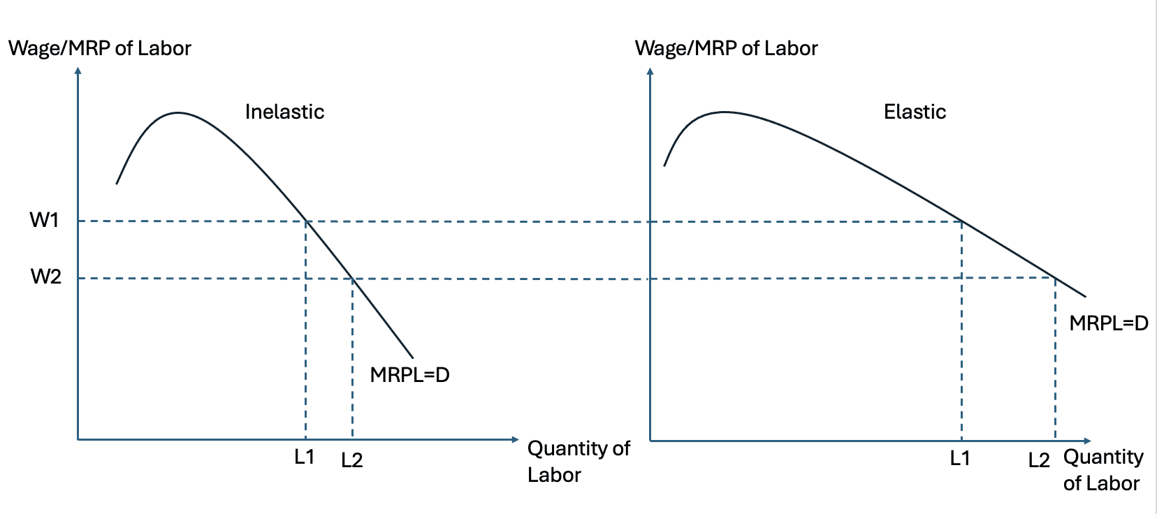
The diagram illustrates two demand curves for labor. The flatter curve shows elastic labor demand—a small rise in the wage causes a large contraction in employment. The steeper curve shows inelastic labor demand—a rise in the wage causes only a small contraction in employment. The difference in slope reflects differences in the underlying determinants of elasticity.

1. Ease of Substituting Labor with Capital or Other Factors

If labor can easily be replaced by capital—such as machines or software—then the demand for labor is likely to be elastic. When the wage rises, firms can quickly switch to cheaper inputs. For example, if production can be automated, the firm may reduce its workforce and increase investment in machinery when labor becomes more expensive. The quantity of labor demanded therefore falls sharply when wages rise.

If labor cannot easily be replaced, labor demand is inelastic. In some tasks, labor and capital are not close substitutes. For example, personal services that require human interaction or creativity may not be easily automated. When the wage rises, the firm has few alternatives and must continue employing roughly the same number of workers. The quantity of labor demanded therefore falls only slightly when wages increase.

The degree of substitutability between labor and capital is therefore one of the strongest determinants of wage elasticity. It determines how flexible the firm can be in changing its input mix when relative factor prices change.

2. Elasticity of Demand for the Final Product

The elasticity of labor demand also depends on how sensitive consumers are to the price of the final product. The reasoning is straightforward. If the wage rises, the firm’s production cost increases. Higher costs push up the product’s price. If consumers are very sensitive to price, they will reduce their purchases significantly. The firm will sell fewer units and therefore need less labor. The demand for labor will be elastic.

If consumers are not very responsive to price, the firm can pass higher wages on to consumers without losing many sales. Output does not fall much, so the firm’s demand for labor is inelastic. The link between product demand elasticity and labor demand elasticity is therefore direct: the more elastic the product demand, the more elastic the derived demand for labor.

This relationship highlights that labor demand is derived. It originates from the demand for output, and its sensitivity to wages depends partly on how strongly output demand reacts to changes in product price.

3. Proportion of Labor Costs in Total Costs

The larger the share of labor costs in total production costs, the more elastic the demand for labor will be. When labor costs form a high proportion of total costs, a given percentage change in wages has a large impact on the firm’s overall costs. This can significantly affect prices and profitability, leading to noticeable adjustments in employment.

When labor costs form a small share of total costs, a change in wages has only a minor effect on total costs. The firm’s profitability and pricing are little affected, so it reduces employment only slightly. Therefore, the higher the proportion of labor costs in total costs, the greater the elasticity of labor demand. The lower that proportion, the less responsive employment is to wage changes.

This determinant explains why wage changes tend to cause large employment adjustments in labor-intensive industries but smaller changes in capital-intensive industries.

4. Time Period Under Consideration

The elasticity of labor demand also depends on the time allowed for adjustment. In the short run, capital and other inputs are often fixed. Firms cannot easily alter their production techniques or invest in new machinery. Because of this rigidity, the demand for labor tends to be inelastic in the short run. When wages rise, firms may continue to employ nearly the same number of workers because they cannot quickly reorganize production.

In the long run, firms have more time to adapt. They can install new machines, change the scale of production, or relocate operations. The possibilities for substituting capital for labor increase, and the demand for labor becomes more elastic. Thus, the longer the time horizon, the greater the ability of firms to adjust their input combinations, and the higher the elasticity of labor demand.

This distinction between short run and long run is central to understanding how employment reacts over time. Short-run rigidities may delay adjustment, while long-run flexibility eventually leads to larger changes in employment.

5. The Mobility and Skills of Labor

Another factor influencing elasticity is the nature of the workforce. If workers are highly skilled and specialized, firms may find it difficult to replace them when wages rise. The demand for such labor is therefore relatively inelastic. If workers are easily replaceable or can be trained quickly, the firm can adjust its employment more readily, making labor demand more elastic.

For example, in an occupation requiring long periods of training, such as engineering or medicine, there may be few available substitutes for experienced workers. Even if wages increase, firms must retain them to maintain operations. Conversely, in occupations where tasks can be performed by workers with minimal training, firms can reduce employment or shift to other inputs more easily when wages rise.

Skill level and labor mobility therefore influence the steepness of the demand curve. Occupations with rare or irreplaceable skills tend to have low wage elasticity of demand, while those with common skills tend to have high wage elasticity.

6. Availability of Raw Materials and Complementary Inputs

Labor productivity and employment depend on the availability of other essential inputs. If these inputs become scarce, labor may add little to output because production is constrained. In that situation, the demand for labor becomes more elastic because the firm cannot justify high wages when the other inputs needed for production are unavailable. Conversely, when complementary inputs are abundant, labor can be used more effectively, and demand becomes less sensitive to wage changes.

For example, if the supply of raw materials required for production becomes restricted, an increase in wages will quickly reduce employment because the firm cannot use labor effectively. When materials are plentiful, a wage increase has less effect on employment because workers remain productive. The same reasoning applies to other complementary factors such as land and capital.

7. Productivity Changes and Expectations About the Future

Expectations about future sales and productivity also affect short-term elasticity. If firms expect output demand to recover soon after a wage rise, they may retain workers even when current wages increase. Employment then appears inelastic in the short run. If firms expect demand to fall further, they may cut labor quickly, leading to high elasticity. Anticipated improvements in productivity can also make firms more tolerant of wage increases, since they expect the marginal revenue product of labor to rise.

These behavioral elements reinforce that elasticity is not fixed. It varies with economic conditions, technology, and expectations.

Labor Productivity and Unit Labor Costs

A firm’s profitability and competitiveness depend on how much output it can produce from its workforce relative to what it pays in wages. Two key measures capture this relationship: labor productivity, which shows how much output each worker produces, and unit labor cost, which shows the labor cost of producing one unit of output. Together, they determine whether the firm’s labor input is efficient and whether it can remain competitive when wages or productivity change.

Labor Productivity

Labor productivity measures the amount of output produced per worker or per hour worked. It is calculated by dividing total output by the number of employees or total hours worked. Productivity reflects how efficiently labor turns inputs into goods and services. It depends on factors such as worker skills and motivation, management quality, technology, capital per worker, and production organization.

When productivity rises, each worker contributes more to output. The marginal physical product of labor increases, and so does the marginal revenue product (MRP), since it equals the marginal physical product multiplied by marginal revenue. The firm can now produce more with the same labor or the same output with fewer workers. This shift increases the value of labor at every wage and moves the MRP curve to the right, raising employment at a given wage.

If productivity falls, the opposite occurs. Each worker produces less, the MRP curve shifts left, and the firm reduces employment to maintain the equality between MRP and the wage. In both cases, the adjustment restores efficiency in labor use.

Unit Labor Costs

Unit labor cost measures the average cost of labor per unit of output. It equals total labor costs divided by total output. A fall in unit labor cost means each unit of output requires less labor expenditure, improving cost competitiveness. A rise means labor has become more expensive relative to its productivity, weakening competitiveness.

Unit labor costs depend on both wage growth and productivity growth.

• If wages rise faster than productivity, unit labor costs increase, raising production costs.

• If productivity grows faster than wages, unit labor costs fall, allowing firms to produce more efficiently.

Productivity, Costs, and Competitiveness

The link between productivity and costs is direct. When productivity improves, the same output can be produced with fewer workers, lowering total labor costs per unit of output. Falling unit labor costs strengthen the firm’s ability to compete. If unit labor costs rise faster than those of competitors, the firm’s relative costs increase—it may need to raise prices or accept lower profits, both of which weaken its position. Conversely, falling unit labor costs give firms an advantage by allowing them to lower prices or expand output profitably.

At the national level, when productivity grows faster than wages, average unit labor costs decline, improving international competitiveness. Exports become cheaper and more attractive, supporting employment and income growth. When wages outpace productivity, unit labor costs rise, prices increase, and competitiveness erodes.

Productivity, Wages, and Employment

Firms continually monitor productivity and labor costs when making hiring decisions. When productivity rises, the marginal revenue product of labor increases, allowing firms to pay higher wages and employ more workers without reducing profits. When productivity stagnates or falls, the MRP declines, and firms must cut wages, raise prices, or reduce employment to remain profitable. Since prices often cannot rise in competitive markets, firms usually respond by reducing labor demand.

Firms therefore have a strong incentive to raise productivity through investment, training, and better management. Sustained productivity growth allows higher real wages and lower prices—both essential for long-term prosperity.

Short-Run and Long-Run Relationships

In the short run, productivity may fluctuate with demand. Unit labor costs can rise temporarily during downturns if firms retain workers despite lower output. In the long run, productivity reflects structural improvements in skills, technology, and capital investment. Maintaining productivity growth that keeps pace with wages is essential for lasting competitiveness and employment growth.

Productivity, Profitability, and Labor Demand

Changes in productivity directly affect labor demand.

• Higher productivity increases the marginal revenue product, shifting the MRP curve outward and allowing higher wages and employment.

• Lower productivity reduces the MRP, shifting it inward and lowering employment at a given wage.

This link between productivity, unit labor costs, and employment ensures that firms hire labor efficiently. Profit maximization occurs where the wage equals the marginal revenue product of labor, aligning employment with productivity and cost conditions.