The Supply of Labor

The analysis of labor markets requires examining not only how firms demand labor but also how individuals choose to supply it. The supply side of the labor market determines how much labor people are willing to offer at various wage levels, and how that willingness combines across individuals to form the total supply to industries and the economy. Understanding labor supply helps explain why the number of hours worked, labor participation, and employment patterns vary as wages change.

The supply of labor refers to the total number of workers or total hours of labor that individuals are prepared to offer to employers at different wage rates. It measures people’s willingness and ability to work, and it is influenced by both economic and social factors. The decision to supply labor involves a trade-off between work and leisure, because each individual must decide how to allocate their time between earning income and enjoying non-working time.

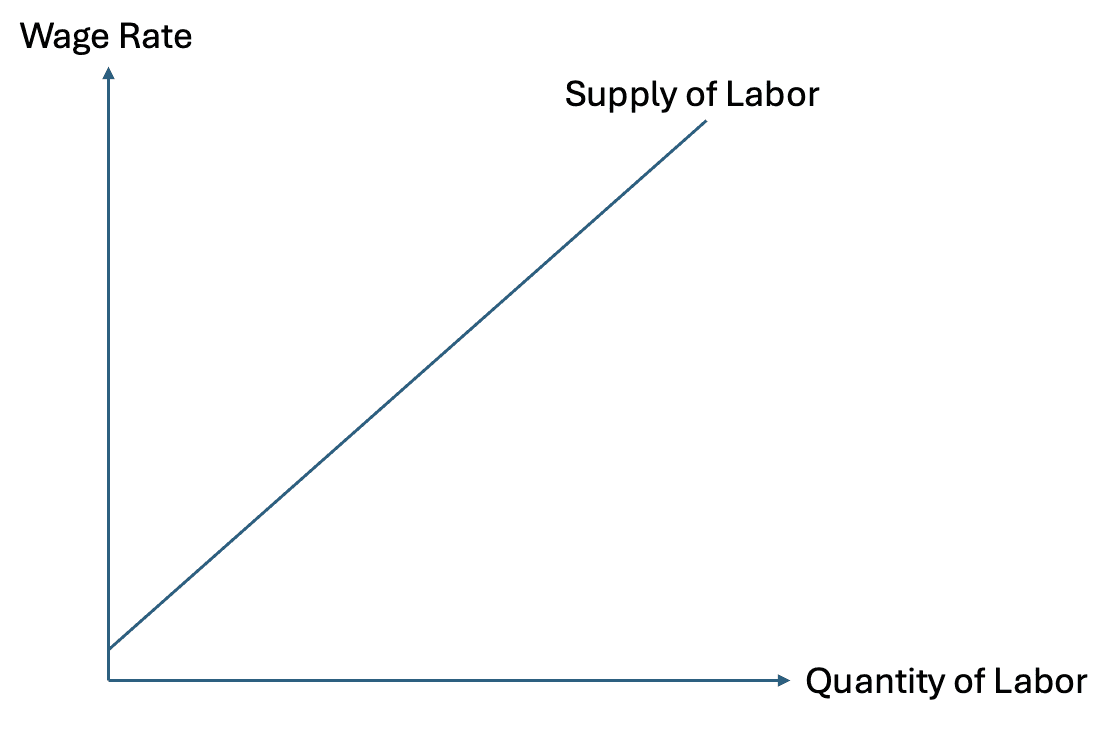
The typical labor supply curve slopes upward from left to right. This shape reflects that higher wages tend to encourage people to work more. As the wage rate rises, work becomes relatively more rewarding compared to leisure, so individuals are willing to offer more hours of labor. However, as will be seen later, this relationship may not always hold at very high wage levels.

The Meaning of Labor Supply in an Industry Context

Labor supply can be considered from two perspectives. The first is the individual worker’s decision, and the second is the aggregate or industry supply that results when many individual decisions are combined.

For an individual, the labor supply decision concerns how many hours they choose to work given the current wage. Each person faces a choice between working to earn income or taking time off for leisure and personal activities. The higher the wage, the greater the reward for each hour worked and the greater the cost of taking time off. The second perspective aggregates these choices across all individuals who might work in a particular occupation, industry, or region. The total labor supplied to that market represents the sum of individual labor hours offered at each wage.

For a single firm operating under perfect competition in the labor market, the supply of labor appears perfectly elastic at the market wage. The firm is too small to influence the overall wage rate and can hire as many workers as it wants at that given wage. In this case, the firm’s labor supply curve is a horizontal line at the market wage, representing a constant marginal cost of labor. However, when examining the supply of labor to an entire industry, the curve is no longer flat. As wages rise, more people are attracted to the industry, and existing workers may offer more hours. Therefore, the industry labor supply curve slopes upward.

The reason for this upward slope is straightforward. A higher wage rate attracts new entrants into the labor market who were previously unwilling to work at lower wages. It also induces existing workers to increase their hours. Conversely, when wages fall, some workers leave the market or cut back their hours, causing the total quantity of labor supplied to fall.

Opportunity Cost of Leisure

The concept of opportunity cost lies at the heart of labor supply decisions. Every hour spent working means an hour not spent on leisure, rest, or personal activities. The opportunity cost of leisure is therefore the income that could have been earned by working instead. Each individual must balance the benefit of additional income against the satisfaction of leisure time.

When the wage rate increases, the opportunity cost of leisure rises because each hour not worked now represents a greater loss of potential earnings. This tends to make leisure more expensive relative to work. As a result, individuals are encouraged to work more and take less leisure. This is known as the substitution effect. It means that a rise in the wage rate causes workers to substitute work for leisure since work has become relatively more rewarding.

However, a second effect operates simultaneously. A higher wage raises a worker’s real income. With higher income, the worker can afford to buy more goods and services, including leisure. If leisure is treated as a normal good, the higher income encourages the worker to take more time off. This is known as the income effect. It pushes in the opposite direction to the substitution effect.

The interaction between these two effects determines how the labor supply curve behaves. At lower wage levels, the substitution effect is usually stronger. Workers are motivated to work more because higher pay makes each hour of work more valuable compared to leisure. At higher wage levels, the income effect may dominate. Since workers already earn enough to meet their goals, further wage increases lead them to value leisure more and to reduce their hours worked.

The Substitution Effect

To understand the substitution effect in more depth, consider an individual who initially earns a moderate wage. When the wage rises, the value of an additional hour worked also rises. Every hour spent on leisure now carries a higher cost in terms of forgone income. Rational workers respond by giving up some leisure and working longer hours to maximize their total income.

In this situation, the individual is said to be substituting work for leisure. The higher wage has changed the relative prices of the two activities, making work relatively cheaper and leisure relatively more expensive. This effect strengthens as the wage continues to increase, drawing more labor into the market.

The substitution effect, therefore, explains the upward-sloping portion of the individual labor supply curve. It dominates at lower and middle wage ranges because most workers value additional income more than the small increase in leisure time that they would gain by reducing their work hours.

The Income Effect

The income effect describes the change in labor supplied that results from a change in real income, holding the relative price of leisure constant. When the wage rate rises, workers feel richer. They can afford to maintain the same level of consumption while enjoying more leisure time. If leisure is a normal good, the higher income will cause workers to demand more leisure and supply less labor.

The income effect works in the opposite direction to the substitution effect. It becomes more important at higher wage levels, where the desire for additional income weakens and the preference for leisure strengthens. Workers may choose to cut their hours, retire early, or move into part-time positions, even though the wage is higher.

The final shape of the labor supply curve depends on which of these effects is stronger. In the lower range of wages, the substitution effect dominates and the curve slopes upward. Beyond a certain wage level, the income effect can offset and eventually outweigh the substitution effect, leading to a backward-bending supply curve.

The Backward-Bending Labor Supply Curve

The backward-bending shape captures how workers’ preferences change as wages become very high. At first, rising wages encourage more labor supply, but beyond a certain point, further increases cause a decline in the number of hours worked.

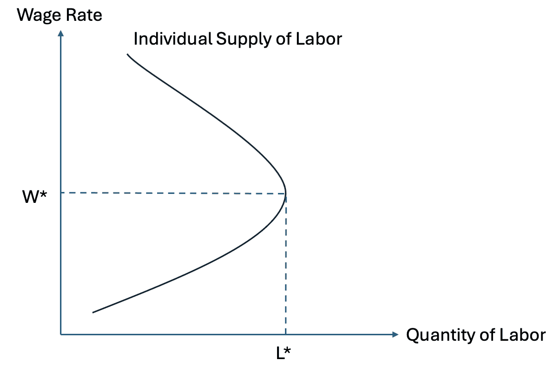
At lower wage levels, workers find it worthwhile to give up leisure to earn more income. As wages rise, they experience an increase in real income and may reach a point where additional income has less value than the leisure it replaces. After that point, the worker reduces labor supplied, creating the backward bend in the curve. The precise turning point varies by individual, depending on preferences for leisure, family circumstances, and lifestyle.

The backward-bending labor supply curve can also represent different stages in life. Younger workers may be strongly motivated by income and career advancement, leading to a steeply upward-sloping supply. Older workers, having achieved a desired standard of living, may prioritize leisure and retire earlier, contributing to the backward bend in the overall labor supply for the economy.

This pattern can also be influenced by taxation, social benefits, and working conditions. For example, high marginal tax rates on additional income can weaken the incentive to work extra hours, reinforcing the income effect and steepening the backward bend. Generous non-wage benefits, such as paid leave or flexible hours, can modify the trade-off between work and leisure in similar ways.

Shifts Versus Movements Along the Labor Supply Curve

It is important to distinguish between a movement along the labor supply curve and a shift of the curve itself. A movement along the curve occurs when the wage rate changes, leading to a change in the quantity of labor supplied. This captures the combined influence of the income and substitution effects discussed above.

A shift in the supply curve, on the other hand, occurs when factors other than the wage change the willingness or ability to work. These include demographic changes, immigration, changes in working conditions, and changes in preferences regarding work-life balance. A rightward shift means that, at every wage, more labor is supplied. A leftward shift means less labor is supplied at every wage.

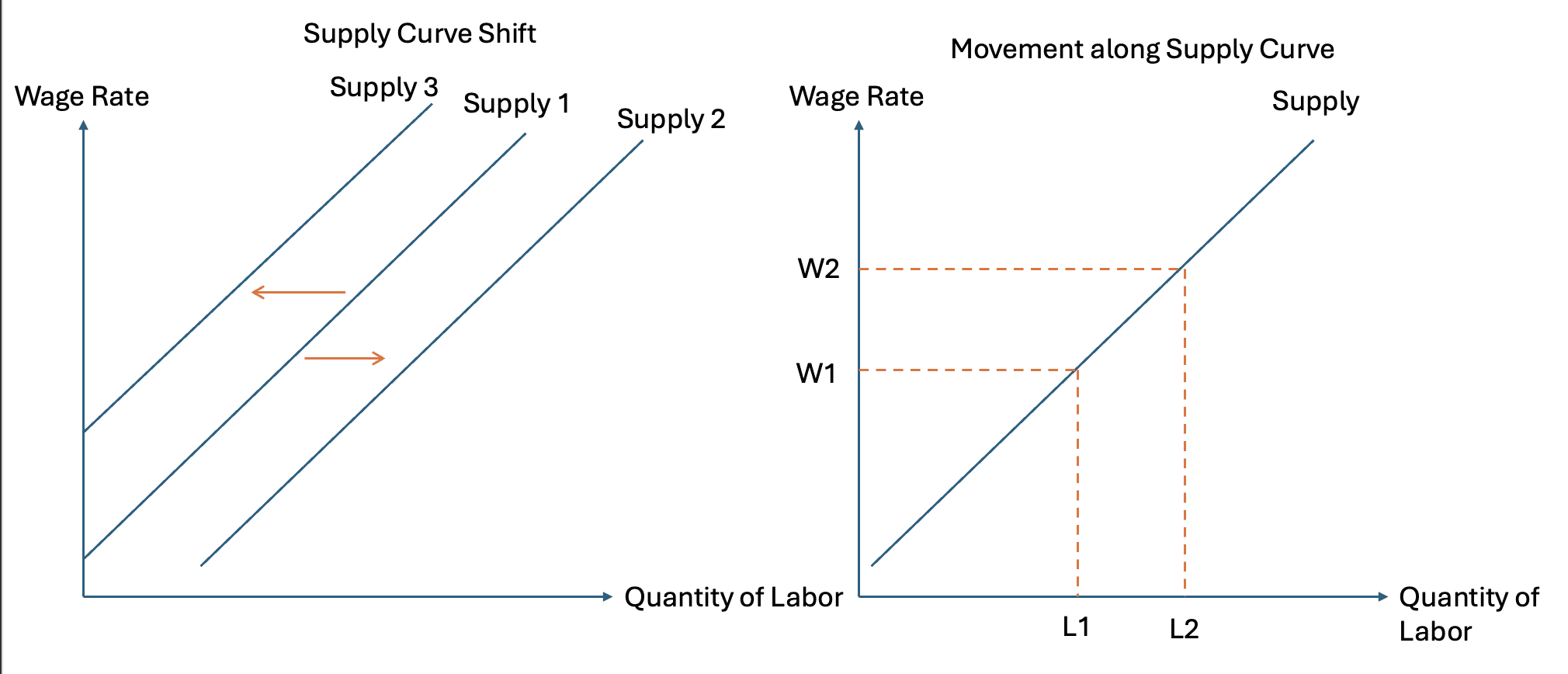
The distinction is crucial because wage changes cause movements along the curve, whereas other factors shift the entire curve.

Factors Influencing the Position of the Labor Supply Curve

The position of the labor supply curve determines how much labor is available to an industry at each possible wage. A change in the wage rate itself causes movement along the supply curve, but when factors other than the wage alter the willingness or ability of workers to supply their labor, the entire curve shifts. These shifts can be either to the right, showing an increase in labor supply at every wage, or to the left, showing a decrease. Understanding these determinants is essential for explaining changes in employment across industries and regions over time.

The labor supply to any given occupation or industry depends on a combination of economic, social, and institutional influences. The most significant factors include wage changes in other industries, differences in skill requirements and qualification costs, the availability of non-monetary job benefits, and demographic trends in the working-age population.

[insert labor supply shift diagram with Wage on vertical axis, Quantity of Labor on horizontal axis, and two upward-sloping curves labeled S₀ and S₁, where S₁ lies to the right showing an increase in labor supply at each wage]

Wages in Other Industries or Occupations

Workers do not make employment decisions in isolation. When the wage offered in one industry changes, workers in other industries may reconsider where to work. If another industry raises its wage, some workers may leave their current occupation to take advantage of better pay elsewhere. This movement reduces the supply of labor to the original industry and shifts its supply curve to the left.

Conversely, if wages fall in a competing industry, workers may move toward the industry that has maintained higher pay, shifting that industry’s supply curve to the right. These inter-industry movements ensure that, over time, wage differences between similar occupations tend to narrow, provided that workers can move freely and that entry requirements are not restrictive.

However, the extent of this movement depends heavily on mobility. If workers require new training, certification, or relocation to switch industries, adjustments occur slowly. Labor markets with greater occupational and geographic mobility experience faster realignment of supply, while those with strong barriers experience persistent differences in wages and employment levels.

Skills and Qualifications

The skills and qualifications required for a job strongly influence labor supply. Occupations that demand advanced skills, lengthy training, or professional credentials tend to have more limited labor supply because fewer people can meet the requirements. These barriers restrict entry and make the supply of labor more inelastic. For example, becoming a qualified engineer, nurse, or pilot involves several years of study and practical training. The cost of obtaining these qualifications discourages some potential workers, narrowing the available supply even if wages rise.

By contrast, occupations that require minimal training or where skills can be learned quickly have more elastic labor supply. When wages increase in such occupations, many new workers can be attracted quickly. This difference in skill barriers helps explain why wage changes lead to much larger employment responses in some industries than in others.

The cost of gaining qualifications also matters. When training programs become cheaper or more accessible, the long-run labor supply expands. Government funding for education or professional licensing can therefore shift the labor supply curve to the right, making the market more flexible and increasing potential employment.

Non-Pecuniary Benefits

Not all influences on labor supply are financial. Non-pecuniary benefits refer to the non-monetary rewards associated with a job that make it more or less attractive to workers. These include job satisfaction, social status, working conditions, job security, training opportunities, flexible hours, and additional perks such as health insurance, pensions, or workplace amenities.

If an occupation offers strong non-pecuniary advantages, workers may accept lower wages in exchange for those benefits. As a result, the labor supply to that industry increases, shifting the supply curve to the right. For example, a job that provides high satisfaction or meaningful work can attract workers even if the pay is modest. Conversely, if working conditions are poor, physically demanding, or dangerous, the labor supply curve shifts left because fewer people are willing to take the job at any given wage.

Fringe benefits and job satisfaction therefore play an important role in determining how labor is distributed across sectors. A profession offering flexible hours and stability may attract workers who value predictability over high income, while high-stress or high-risk jobs may need to offer wage premiums to offset their disadvantages. These compensating wage differentials are an essential feature of labor market equilibrium, balancing monetary and non-monetary rewards across occupations.

Demographic Factors

The demographic composition of the population affects the overall availability of labor. The total number of people in the working-age group determines the potential size of the labor force. Changes in population growth, aging, immigration, and participation rates all influence the aggregate labor supply.

An increase in the working-age population, for example through immigration or higher birth rates, shifts the total labor supply curve to the right. Conversely, an aging population or declining participation rate shifts it to the left. The participation rate measures the proportion of people of working age who are either employed or actively seeking work. When participation falls due to early retirement, prolonged education, or social norms discouraging certain groups from working, the total labor supply contracts.

Immigration is an especially significant factor in labor markets. When new workers enter a country, they expand the potential workforce, particularly in occupations where domestic labor is scarce. This can ease labor shortages and moderate wage pressures. However, if immigration is concentrated in certain sectors, it can temporarily push wages down in those industries. The overall impact depends on how quickly the economy absorbs new workers and on whether their skills complement or substitute for native workers.

Demographic structure also influences labor supply indirectly through education and gender participation. Rising female participation rates, delayed retirement, and expanding higher education each reshape the pattern of labor availability across sectors and time. For example, if more people pursue university degrees, the long-term supply of skilled labor increases, while the short-term supply of unskilled labor may tighten. These changes illustrate why labor supply dynamics must be analyzed over both short and long horizons.

The Role of Job-Specific Conditions and Mobility

Geographic and occupational mobility are closely linked to the responsiveness of labor supply. Geographic mobility refers to workers’ ability and willingness to move to different regions for employment. Occupational mobility refers to their ability to switch industries or roles that require different skills. If workers can move freely across locations or occupations, labor supply is more elastic, since wage differences can quickly attract new entrants.

In contrast, when mobility is restricted by housing costs, family commitments, or legal barriers, the labor supply becomes inelastic. Even significant wage changes may fail to attract enough workers to fill vacancies. This immobility is especially evident in specialized professions or in regions with limited transport and high relocation costs.

Mobility also interacts with time. In the short run, workers are less able to retrain or relocate, so labor supply tends to be inelastic. Over the long run, as people adjust and gain new skills, supply becomes more elastic. This distinction between short-run and long-run responses helps explain why industries facing sudden demand surges often experience temporary labor shortages that diminish over time as more workers enter the field.

Government intervention

Labor supply can also be affected by institutional arrangements such as unions, professional licensing, and government regulation. Trade unions can restrict or expand labor supply depending on their objectives. By limiting membership or imposing entry requirements, they can reduce the number of workers eligible for certain jobs, shifting the supply curve leftward and maintaining higher wages for existing members. On the other hand, unions may also negotiate for better working conditions or training schemes that attract more workers, shifting the curve to the right.

Similarly, government policies concerning working hours, retirement age, and social benefits affect labor availability. Increasing the retirement age or reducing unemployment benefits may encourage greater participation, while generous welfare provisions or early retirement incentives may reduce labor supply at given wage levels.

Institutional influences are particularly significant in the public sector, where wages are often set administratively rather than through market competition. Policy reforms can therefore shift supply dramatically without any change in the underlying market wage.

Short-Run and Long-Run Adjustments in Labor Supply

In the short run, the number of workers available to an industry is constrained by existing training levels, geographic distribution, and current employment. If demand for labor increases suddenly, wages may rise sharply because the short-run supply is inelastic. Over time, new workers are trained or attracted into the occupation, and the supply curve gradually shifts to the right, moderating the wage increase.

This gradual response explains why wages can remain elevated for several years in industries experiencing strong growth, such as technology or healthcare, until new entrants expand the labor pool. Conversely, when demand falls, supply may not contract immediately, leading to temporary unemployment or underemployment. Over time, workers retrain or exit the industry, restoring equilibrium at a lower wage.

The Wage Elasticity of Labor Supply

The wage elasticity of labor supply measures how strongly the quantity of labor supplied responds to a change in the wage rate. It captures the degree of flexibility in the labor market, showing whether workers adjust their hours, participation, or occupation quickly when wages rise or fall. A clear understanding of this concept is vital because it affects how wages influence employment, migration, and overall labor market balance.

Elasticity in this context expresses responsiveness as a ratio of percentage changes. It is calculated as the percentage change in the quantity of labor supplied divided by the percentage change in the wage rate. When the absolute value of this ratio is greater than one, labor supply is said to be elastic, meaning workers respond strongly to wage changes. When the absolute value is less than one, labor supply is inelastic, meaning that changes in wages produce only small changes in the amount of labor supplied.

The elasticity of labor supply is not constant. It varies across industries, occupations, and time periods. It depends on how easily people can enter or leave particular jobs, how long it takes to train, and what other opportunities exist. Several key determinants explain these differences and help to predict whether labor supply will respond sharply or slowly to a change in wages.

Availability of Workers

The availability of workers refers to how many people are ready and able to take jobs in a given occupation when wages change. When a large pool of potential workers exists, labor supply tends to be elastic. Even a modest wage increase can attract new participants from unemployment, part-time work, or other sectors.

If unemployment is high, many people are already seeking jobs. A small rise in the wage will quickly draw them into employment, leading to a large percentage increase in the quantity of labor supplied. In contrast, when the economy is near full employment, few additional workers remain available. A rise in wages then brings only a limited increase in supply. The labor market in that case is inelastic because nearly everyone willing to work is already employed.

The availability of workers therefore plays a central role in explaining why labor supply tends to be more elastic during recessions, when spare labor exists, and less elastic during booms, when labor markets are tight.

Skills

Skill requirements strongly affect labor supply elasticity. When a job requires specialized training or experience, the pool of qualified candidates is small. As a result, even a significant increase in wages may not quickly attract new workers, because others lack the required skills. Labor supply in such occupations is inelastic.

For example, professions such as medicine or aviation require long training periods. If the wage for pilots or doctors rises, it may take many years for new entrants to complete training and expand the labor force. Conversely, when a job requires minimal training, workers can move into it rapidly, making supply elastic.

Skill barriers therefore determine how responsive labor supply is to wage incentives. When skill acquisition is costly or time-consuming, the short-run elasticity is low. Over the long run, however, training programs and education can increase the number of qualified workers, gradually making the supply more elastic.

Qualifications

Qualifications are closely linked to skills but emphasize formal certification or licensing. Many professional jobs require official qualifications such as degrees, apprenticeships, or government licenses. The more extensive or costly these qualifications are, the smaller the number of people who can enter the profession at short notice.

In fields like accountancy or law, years of education and examinations restrict entry, limiting the elasticity of supply. A rise in wages may encourage more students to pursue these careers, but the adjustment happens slowly because qualification takes time. In occupations where no official qualifications are needed, entry is easier and elasticity higher.

This distinction also applies internationally. Occupations requiring qualifications recognized only in one country tend to have low short-run elasticity because foreign workers cannot immediately join the workforce. Policies that make foreign credentials transferable can raise long-run elasticity by expanding the available pool of qualified labor.

Labor Immobility

Labor immobility refers to obstacles preventing workers from moving freely between jobs or locations. It can be geographic, meaning difficulty in relocating to another region, or occupational, meaning difficulty in switching to another type of work. Immobility reduces elasticity because workers cannot easily respond to wage changes elsewhere.

If a wage increase occurs in a different city, but high housing costs or family commitments make relocation difficult, few workers will move to take advantage of it. The labor supply in that city remains inelastic. Likewise, if an occupation demands skills that are not easily transferable, workers cannot shift occupations quickly. High occupational immobility therefore keeps elasticity low even when wages change sharply.

In the long run, geographic mobility can increase as housing markets adjust and transport links improve. Similarly, occupational mobility can improve with retraining opportunities. The elasticity of labor supply thus depends not only on immediate conditions but also on the capacity of workers and institutions to adapt over time.

Short-Run and Long-Run Elasticity

In the short run, the number of people who can respond to a wage change is limited. Workers are tied to existing jobs, housing, and skills. Firms that raise wages cannot immediately attract a large number of new employees because few are available. Short-run labor supply is therefore relatively inelastic.

Over the long run, workers can make adjustments. They can acquire new skills, relocate, or change occupations. Younger generations may choose training paths that align with higher wages in growing industries. These gradual changes make labor supply more elastic in the long term.

The distinction between short and long horizons explains why industries experiencing sudden surges in demand often face temporary shortages and rising wages, while the same industries later stabilize as new workers enter. For example, a sharp increase in wages for software engineers may not immediately produce more engineers, but over several years, educational institutions expand programs and more students train in that field, increasing supply.

The Impact of Unemployment and Underemployment

The presence of unemployment or underemployment increases the elasticity of labor supply. When there are many workers without jobs or with part-time jobs who would prefer full-time work, a wage increase quickly draws them into employment. The supply response is large because these individuals do not need to acquire new skills or relocate.

In contrast, when the economy operates close to full capacity, nearly everyone who wants to work already has a job. Additional wage increases cannot attract many new workers, so elasticity is low. In this way, the cyclical state of the economy affects short-term responsiveness.

Institutional and Social Influences

The structure of labor institutions also affects how elastic supply is. In countries or sectors with strong unions, collective agreements may limit the flexibility of hours or participation. Even if wages rise, union rules or fixed schedules can restrict labor supply, keeping elasticity low.

Social factors such as cultural attitudes toward work, gender roles, or family responsibilities can also shape elasticity. For instance, in societies where part-time or flexible work options are common, a small wage change can encourage more people to join the labor market. Where social norms discourage participation, particularly among certain groups, elasticity remains low regardless of wage movements.

Over time, cultural and institutional changes can modify these patterns. The expansion of childcare facilities, remote work technology, or equal opportunity policies often increases the elasticity of labor supply by removing non-wage barriers to participation.

Differences Between Occupations

Elasticity also varies systematically between different types of jobs. In routine, low-skill occupations where workers can be replaced or trained quickly, supply is highly elastic. A small wage rise can attract many new entrants. In contrast, in specialized professions or in jobs requiring long-term commitment, such as medicine, architecture, or academia, supply is much less responsive.

This difference helps to explain why wage increases in some industries lead to large employment growth while in others they lead mostly to higher earnings without significant increases in employment. It also underlies structural differences in income distribution across sectors.

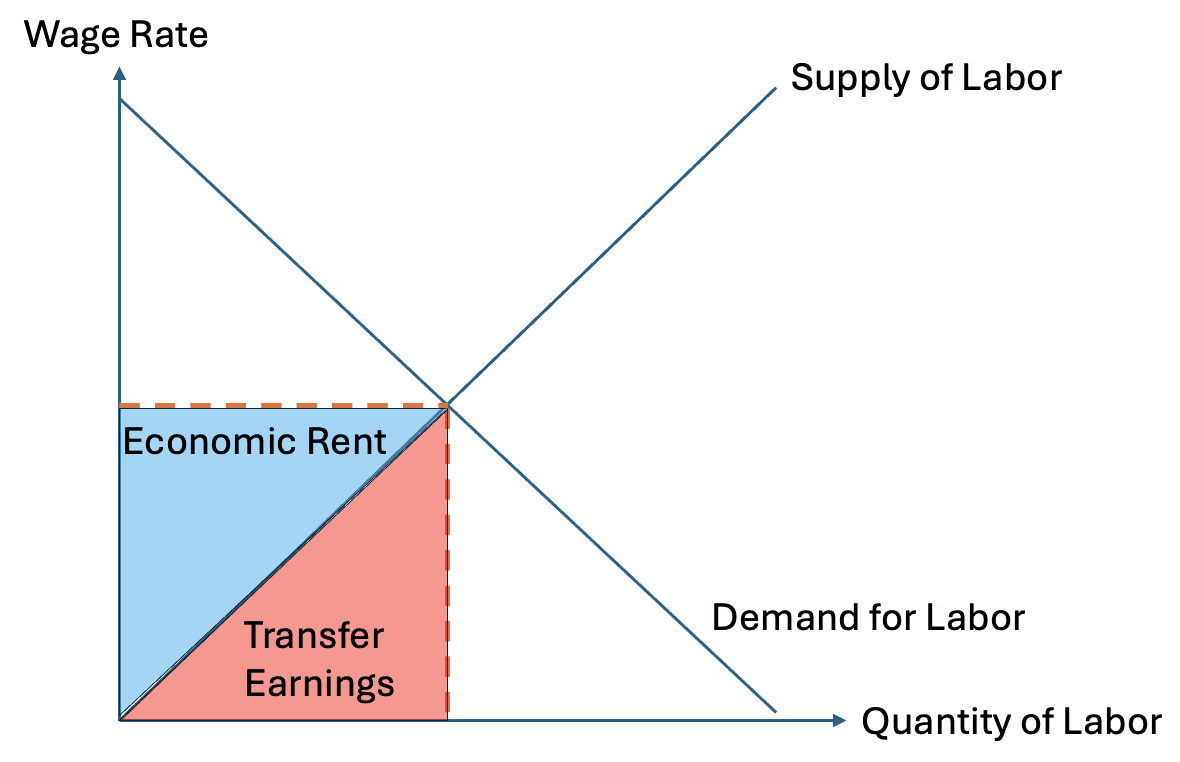
Transfer Earnings and Economic Rent

When analyzing labor markets, economists often want to know how much of a worker’s wage is the minimum payment needed to keep that worker in the current job and how much represents an extra reward above that minimum. To make this distinction clear, two important ideas are used: transfer earnings and economic rent.

Transfer earnings represent the minimum payment required to keep a factor of production, such as labor, in its current use. Economic rent represents any additional payment a worker receives above this minimum. The combination of both makes up the worker’s total earnings.

Understanding how wages divide between transfer earnings and economic rent provides insight into labor market efficiency, occupational differences, and income inequality. It also shows how the elasticity of labor supply affects the share of each component.

Defining Transfer Earnings

Transfer earnings can be defined as the minimum income a worker must receive to remain employed in a given occupation. If a worker could earn a certain wage in another job, that alternative wage is the worker’s transfer earning. It reflects the opportunity cost of keeping the worker in the current role.

In simple terms, transfer earnings measure what the worker would need to be paid to prevent them from leaving for another job. If the current wage falls below this amount, the worker will leave because they can earn more elsewhere.

Transfer earnings therefore depend on alternative opportunities. Workers with many options, such as general administrative staff, tend to have higher transfer earnings because other employers are ready to hire them at similar wages. Workers with fewer alternatives, such as those in specialized roles or in locations with limited job openings, have lower transfer earnings because they have fewer competing opportunities.

Defining Economic Rent

Economic rent is the extra income a factor of production earns above the minimum required to keep it in its current use. For labor, it represents the portion of wages that exceeds the worker’s transfer earnings.

This surplus arises because some workers possess scarce skills, talents, or attributes that make them more productive or harder to replace. For example, a surgeon, professional athlete, or top software engineer may receive wages well above the minimum they would accept because their unique abilities create high value for employers.

Economic rent therefore reflects the reward for scarcity or exceptional productivity. It is not determined by necessity but by market conditions that allow certain workers to command pay above the going rate needed to retain them.

Relationship Between the Two Concepts

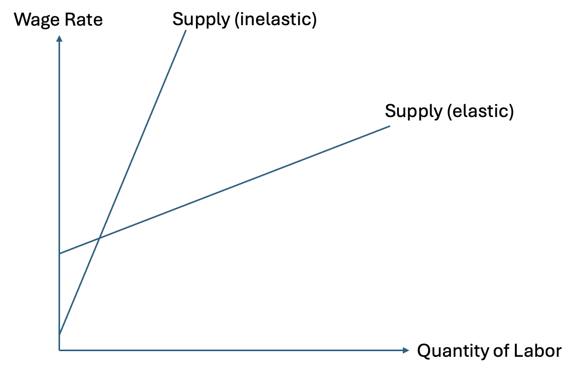
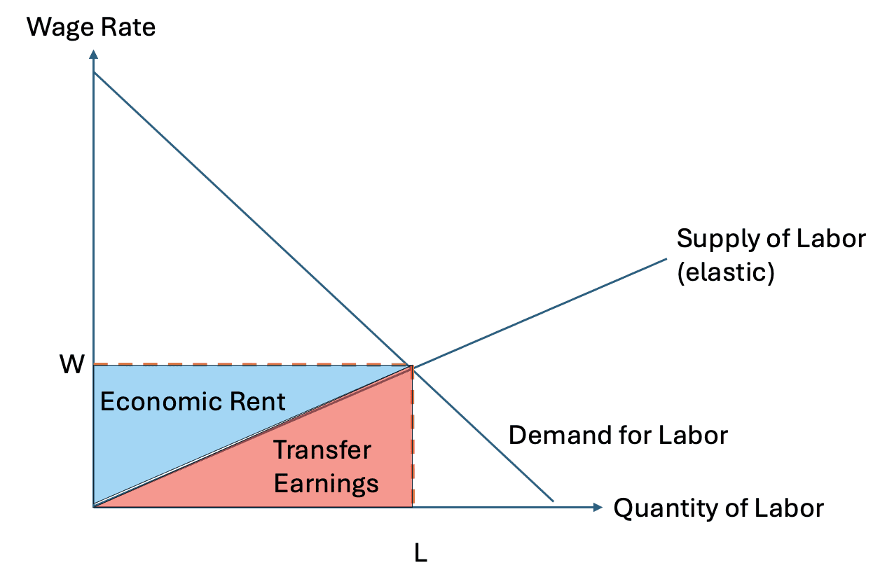
A worker’s total wage equals transfer earnings plus economic rent. The size of each component depends on the shape of the labor supply curve. When supply is perfectly elastic, wages are determined by the market, and every worker earns exactly their transfer earnings with no economic rent. When supply is perfectly inelastic, all payments to labor are economic rent because no alternative opportunity is required to keep workers in employment.

This diagram shows that as the supply of labor becomes less elastic, a greater proportion of total earnings becomes economic rent. When the supply curve is steep, wages can rise significantly without attracting much additional labor, creating a large surplus for existing workers. When the supply curve is flat, any attempt to raise wages quickly attracts new workers, leaving little room for rent.

How Transfer Earnings Arise

To see how transfer earnings operate, imagine a worker who could earn twenty pounds per hour as a technician in one firm or a similar amount in another. The twenty-pound rate is their opportunity cost. If the current employer offers less than that, the worker will leave. If the employer offers exactly twenty pounds, the worker stays but earns no surplus above the minimum.

Transfer earnings therefore set the floor for acceptable wages. They are determined not by the current employer but by the next best alternative available to the worker. Changes in outside opportunities, such as new job openings or regional growth, can raise or lower transfer earnings across the economy.

When many firms compete for the same type of worker, transfer earnings rise because workers have multiple alternatives. When jobs are scarce, transfer earnings fall because options are limited and workers will stay even for lower pay. These shifts influence the minimum necessary wage in each market.

How Economic Rent Arises

Economic rent arises when a worker’s abilities or circumstances prevent easy replacement. If the supply of a particular skill is limited, employers must pay well above the minimum necessary to secure those workers. The extra payment above transfer earnings becomes economic rent.

This surplus can be temporary or long-lasting. In the short run, sudden changes in demand for specific skills can generate rent until more workers are trained. In the long run, if training expands and more people acquire those skills, competition reduces the rent component.

Economic rent is also influenced by natural talent, exceptional performance, or barriers to entry. For instance, only a few athletes can play at the highest professional level. Their wages include very large economic rents because the supply of comparable talent is nearly fixed. In contrast, wages in occupations with many equally qualified workers include little or no rent.

Elasticity of Supply and Its Effects

The elasticity of the labor supply curve determines how wages are divided between transfer earnings and rent.

When labor supply is perfectly elastic, the curve is horizontal. The wage is fixed by the market, and all workers are paid exactly what they require to stay in employment. There is no rent because new workers can enter freely at the same wage.

When labor supply is perfectly inelastic, the curve is vertical. The quantity of labor is fixed, and workers cannot increase or decrease their supply regardless of wage changes. The entire wage payment is therefore economic rent, since no alternative wage is necessary to retain labor.

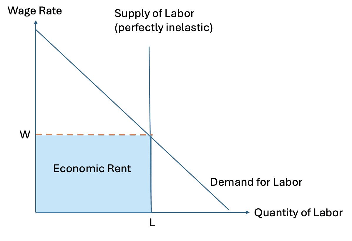
Between these two extremes lie the real-world cases. Occupations with steep, inelastic supply curves such as surgeons, top scientists, or elite athletes generate significant rent. Occupations with flat, elastic supply curves such as retail workers or call-center employees generate little rent because many substitutes exist.

Connection to Opportunity Cost

The concept of transfer earnings is rooted in opportunity cost. Every worker faces a choice between current employment and the next best alternative. The transfer earning equals the opportunity cost of staying in the present job. Economic rent is the difference between actual wage and that opportunity cost.

This connection helps explain how labor reallocates across markets. When an alternative job offers higher pay, opportunity cost rises, reducing economic rent in the current job. Workers may switch positions until wages reflect opportunity costs across the market. The continuous movement of workers in response to these differences helps equalize returns in the long run.

Income Distribution and Policy Implications

The distinction between transfer earnings and economic rent has policy significance. Taxes on economic rent do not distort labor allocation because rent does not affect the decision to work. However, taxes that reduce transfer earnings can discourage labor supply by lowering the minimum payment required to retain workers.

Similarly, when wage controls or union negotiations push wages above equilibrium, they can increase the rent component but may reduce employment. Understanding which part of income is rent helps policymakers design taxes and labor regulations that minimize inefficiency.